
Methodology, Parameters, and Calculations
Parameter definitions, formulas, uncertainty ranges, and data sources.
Keywords
health economics methodology, clinical trial cost analysis, medical research ROI, cost-benefit analysis healthcare, sensitivity analysis, Monte Carlo simulation, DALY calculation, pragmatic clinical trials
Overview
This appendix documents all 74 parameters used in the analysis, organized by type:
- External sources (peer-reviewed): 27
- Calculated values: 30
- Core definitions: 17
Calculated Values
Parameters derived from mathematical formulas and economic models.
Current Trajectory Average Income at Year 20: $20.5K
Note📊 Details
Average income (GDP per capita) at year 20 under current trajectory trajectory.
Inputs:
- Current Trajectory GDP at Year 20 🔢: $188T
- Global Population 2045 (Projected) 📊: 9.2 billion of people
\[ \begin{gathered} \bar{y}_{base,20} \\ = \frac{GDP_{base,20}}{Pop_{2045}} \\ = \frac{\$188T}{9.2B} \\ = \$20.5K \end{gathered} \] where: \[ GDP_{base,20} = GDP_0(1+g_{base})^{20} \] ✓ High confidence
Monte Carlo Distribution
Simulation Results Summary: Current Trajectory Average Income at Year 20
| Statistic | Value |
|---|---|
| Baseline (deterministic) | $20.5K |
| Mean (expected value) | $20.5K |
| Median (50th percentile) | $20.5K |
| Standard Deviation | $3.64e-12 |
| 90% Range (5th-95th percentile) | [$20.5K, $20.5K] |
The histogram shows the distribution of Current Trajectory Average Income at Year 20 across 10,000 Monte Carlo simulations. The CDF (right) shows the probability of the outcome exceeding any given value, which is useful for risk assessment.
Exceedance Probability
This exceedance probability chart shows the likelihood that Current Trajectory Average Income at Year 20 will exceed any given threshold. Higher curves indicate more favorable outcomes with greater certainty.
Current Trajectory GDP at Year 20: $188T
Note📊 Details
Global GDP at year 20 under status-quo current trajectory growth.
Inputs:
- Global GDP (2025) 📊: $115T
- Baseline Global GDP Growth Rate: 2.5%
\[ GDP_{base,20} = GDP_0(1+g_{base})^{20} \]
✓ High confidence
Monte Carlo Distribution
Simulation Results Summary: Current Trajectory GDP at Year 20
| Statistic | Value |
|---|---|
| Baseline (deterministic) | $188T |
| Mean (expected value) | $188T |
| Median (50th percentile) | $188T |
| Standard Deviation | $0.031 |
| 90% Range (5th-95th percentile) | [$188T, $188T] |
The histogram shows the distribution of Current Trajectory GDP at Year 20 across 10,000 Monte Carlo simulations. The CDF (right) shows the probability of the outcome exceeding any given value, which is useful for risk assessment.
Exceedance Probability
This exceedance probability chart shows the likelihood that Current Trajectory GDP at Year 20 will exceed any given threshold. Higher curves indicate more favorable outcomes with greater certainty.
Total Annual Decentralized Framework for Drug Assessment Operational Costs: $40M
Note📊 Details
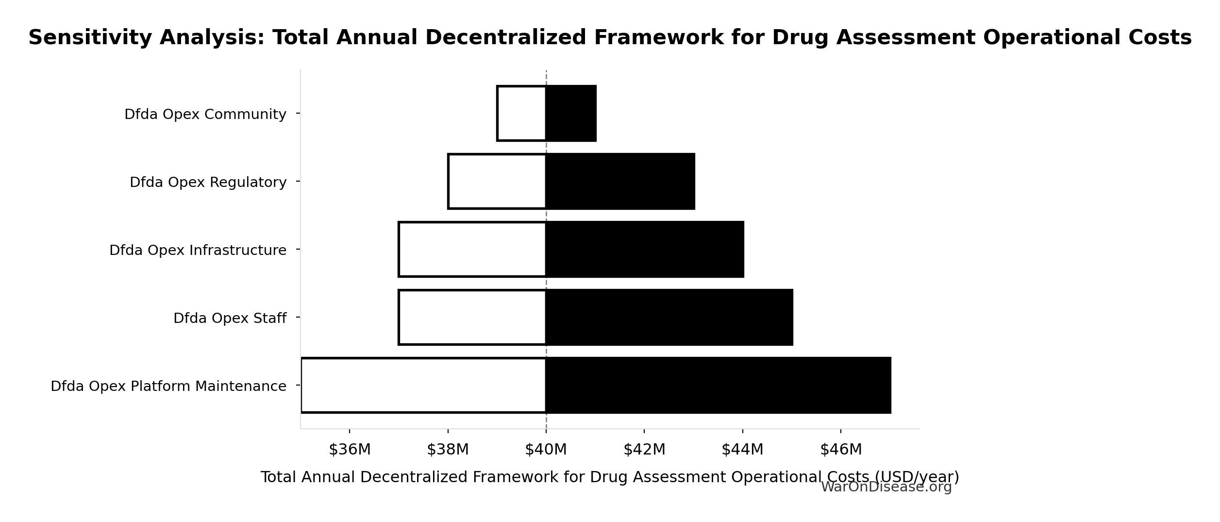
Total annual Decentralized Framework for Drug Assessment operational costs (sum of all components: platform + staff + infra + regulatory + community)
Inputs:
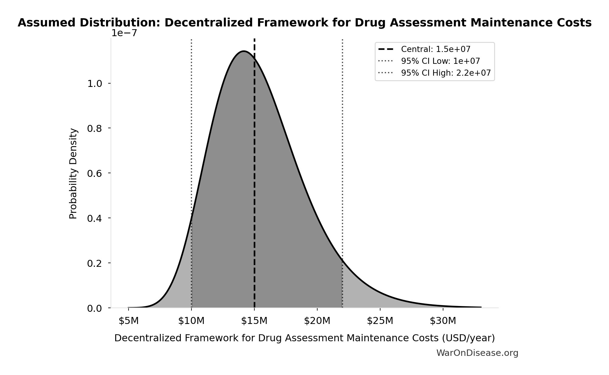
- Decentralized Framework for Drug Assessment Maintenance Costs: $15M (95% CI: $10M - $22M)
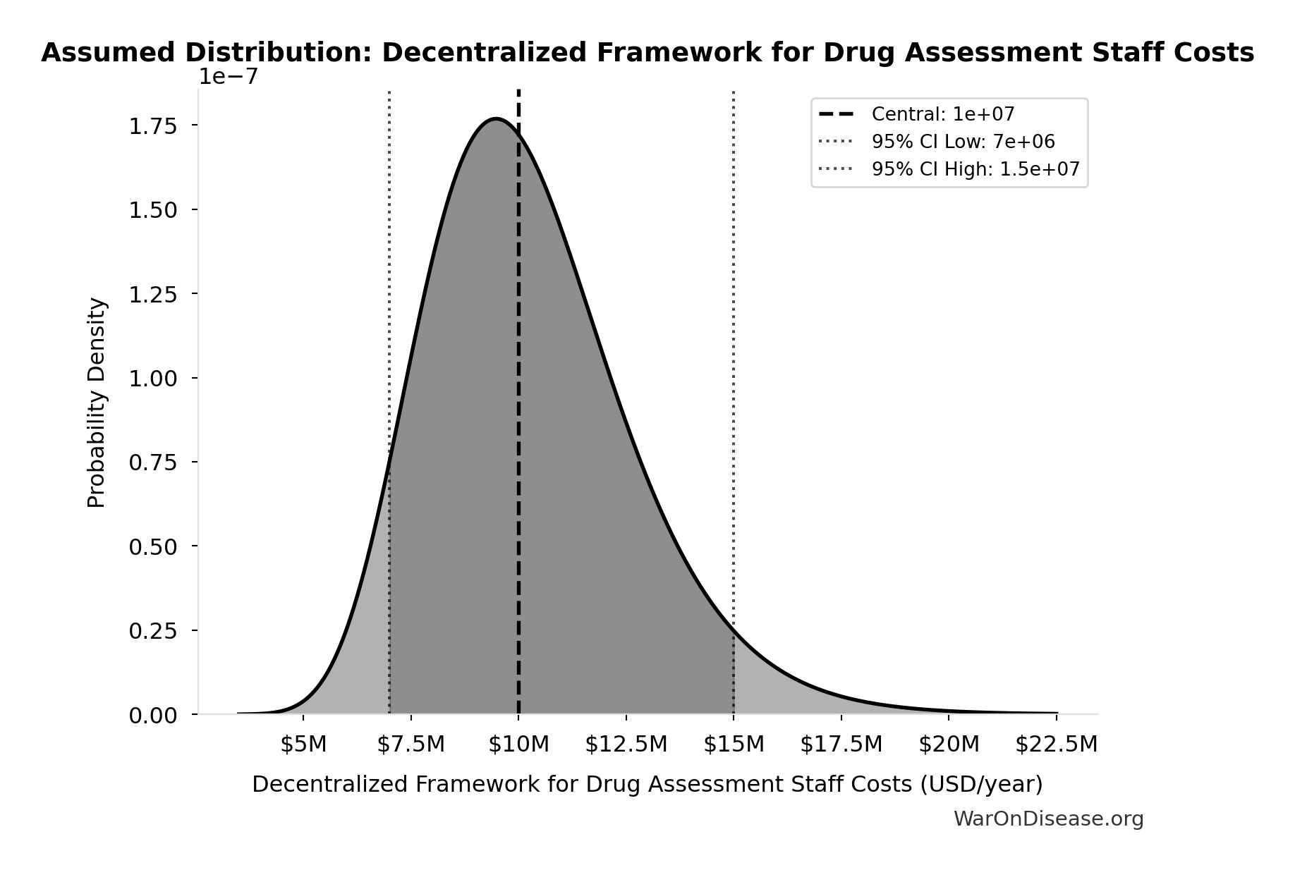
- Decentralized Framework for Drug Assessment Staff Costs: $10M (95% CI: $7M - $15M)
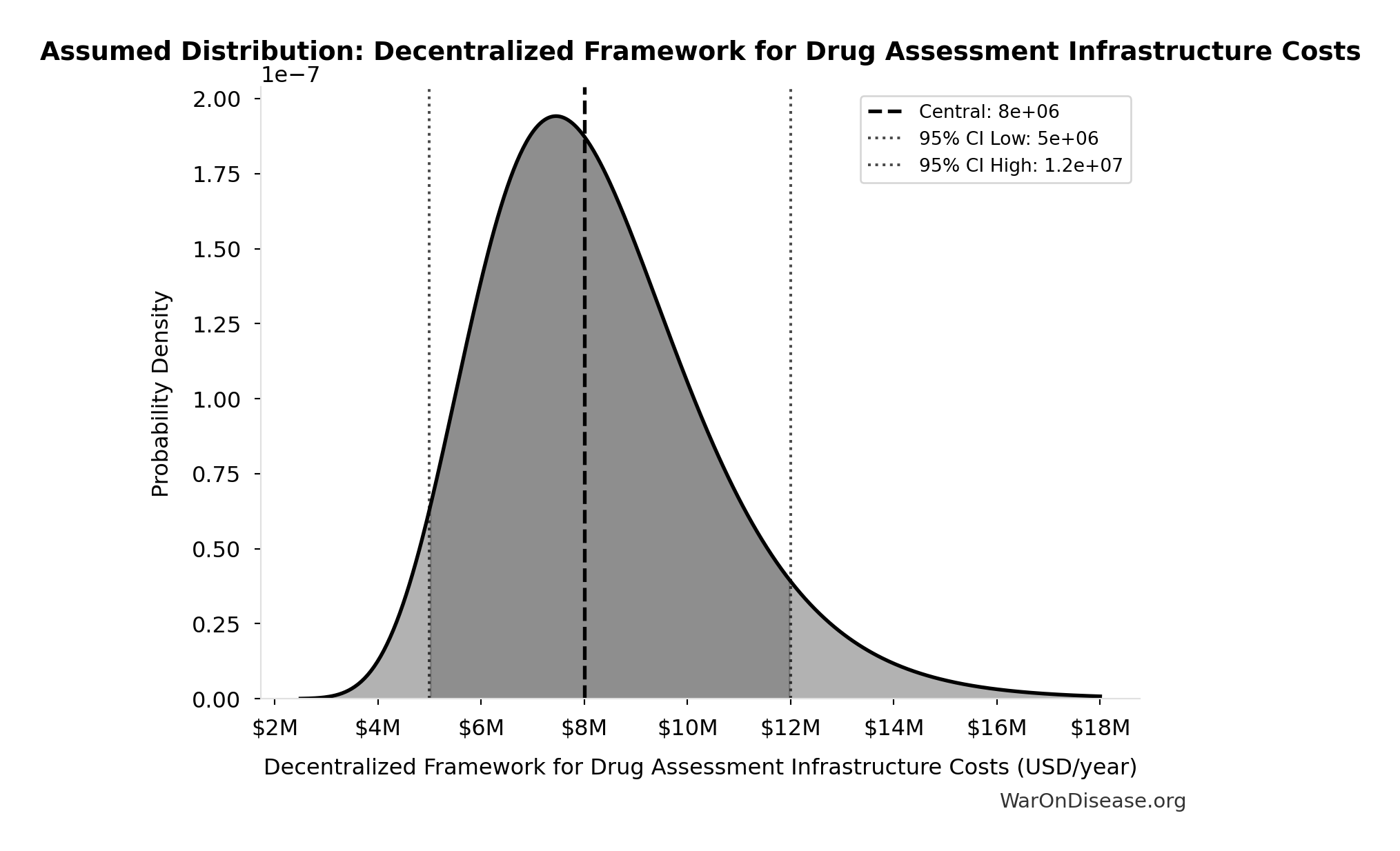
- Decentralized Framework for Drug Assessment Infrastructure Costs: $8M (95% CI: $5M - $12M)
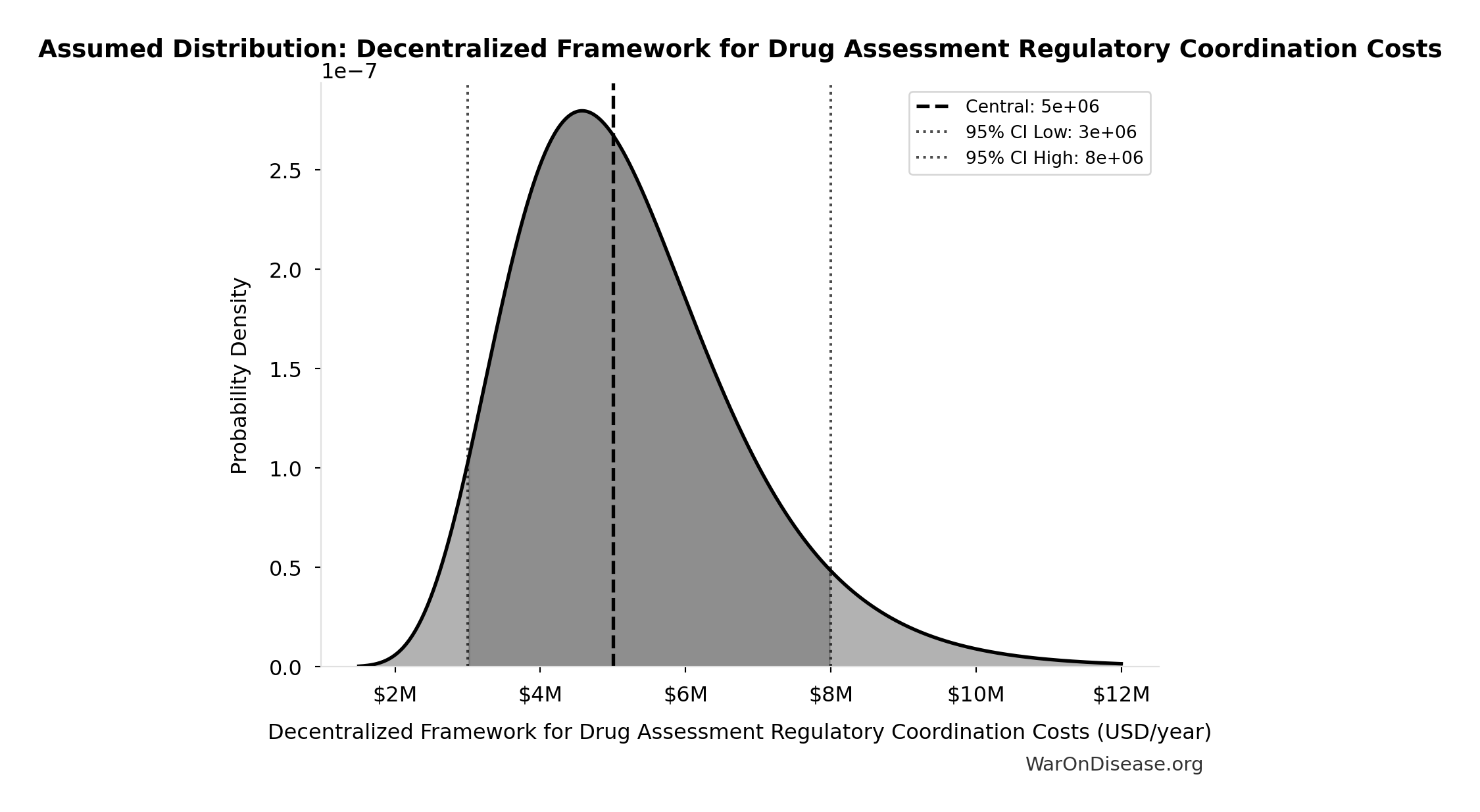
- Decentralized Framework for Drug Assessment Regulatory Coordination Costs: $5M (95% CI: $3M - $8M)
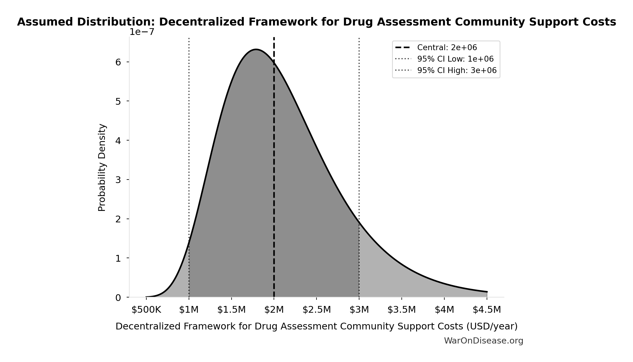
- Decentralized Framework for Drug Assessment Community Support Costs: $2M (95% CI: $1M - $3M)
\[ \begin{gathered} OPEX_{dFDA} \\ = Cost_{platform} + Cost_{staff} + Cost_{infra} \\ + Cost_{regulatory} + Cost_{community} \\ = \$15M + \$10M + \$8M + \$5M + \$2M \\ = \$40M \end{gathered} \]
✓ High confidence
Sensitivity Analysis
Sensitivity Indices for Total Annual Decentralized Framework for Drug Assessment Operational Costs
Regression-based sensitivity showing which inputs explain the most variance in the output.
| Input Parameter | Sensitivity Coefficient | Interpretation |
|---|---|---|
| Decentralized Framework for Drug Assessment Maintenance Costs (USD/year) | 0.3542 | Moderate driver |
| Decentralized Framework for Drug Assessment Staff Costs (USD/year) | 0.2355 | Weak driver |
| Decentralized Framework for Drug Assessment Infrastructure Costs (USD/year) | 0.2060 | Weak driver |
| Decentralized Framework for Drug Assessment Regulatory Coordination Costs (USD/year) | 0.1469 | Weak driver |
| Decentralized Framework for Drug Assessment Community Support Costs (USD/year) | 0.0576 | Minimal effect |
Interpretation: Standardized coefficients show the change in output (in SD units) per 1 SD change in input. Values near ±1 indicate strong influence; values exceeding ±1 may occur with correlated inputs.
Monte Carlo Distribution
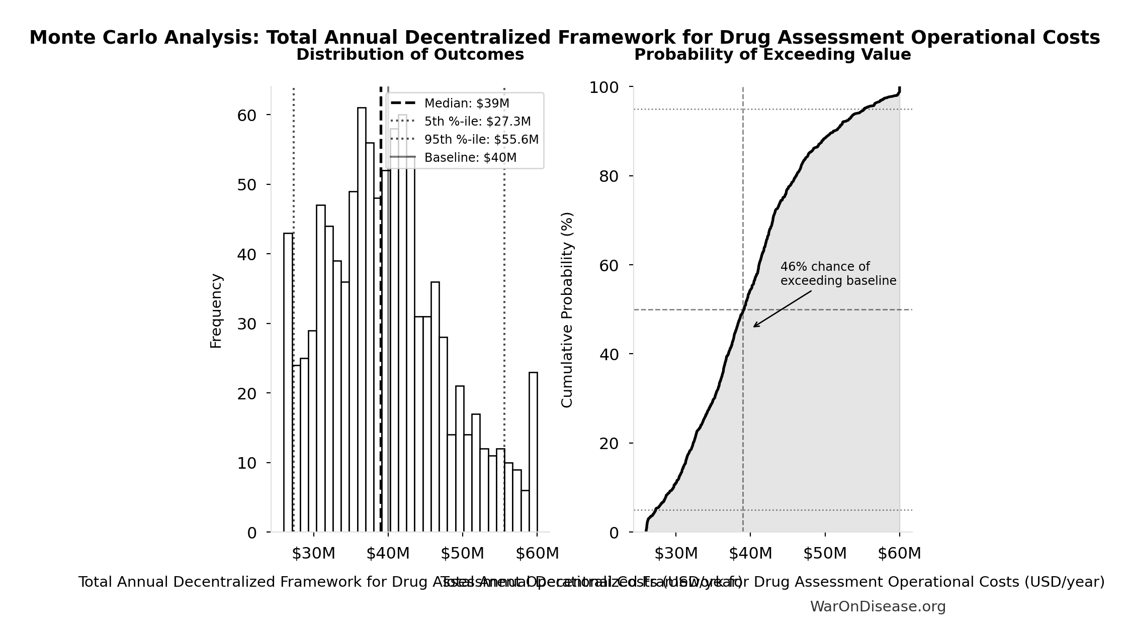
Simulation Results Summary: Total Annual Decentralized Framework for Drug Assessment Operational Costs
| Statistic | Value |
|---|---|
| Baseline (deterministic) | $40M |
| Mean (expected value) | $39.9M |
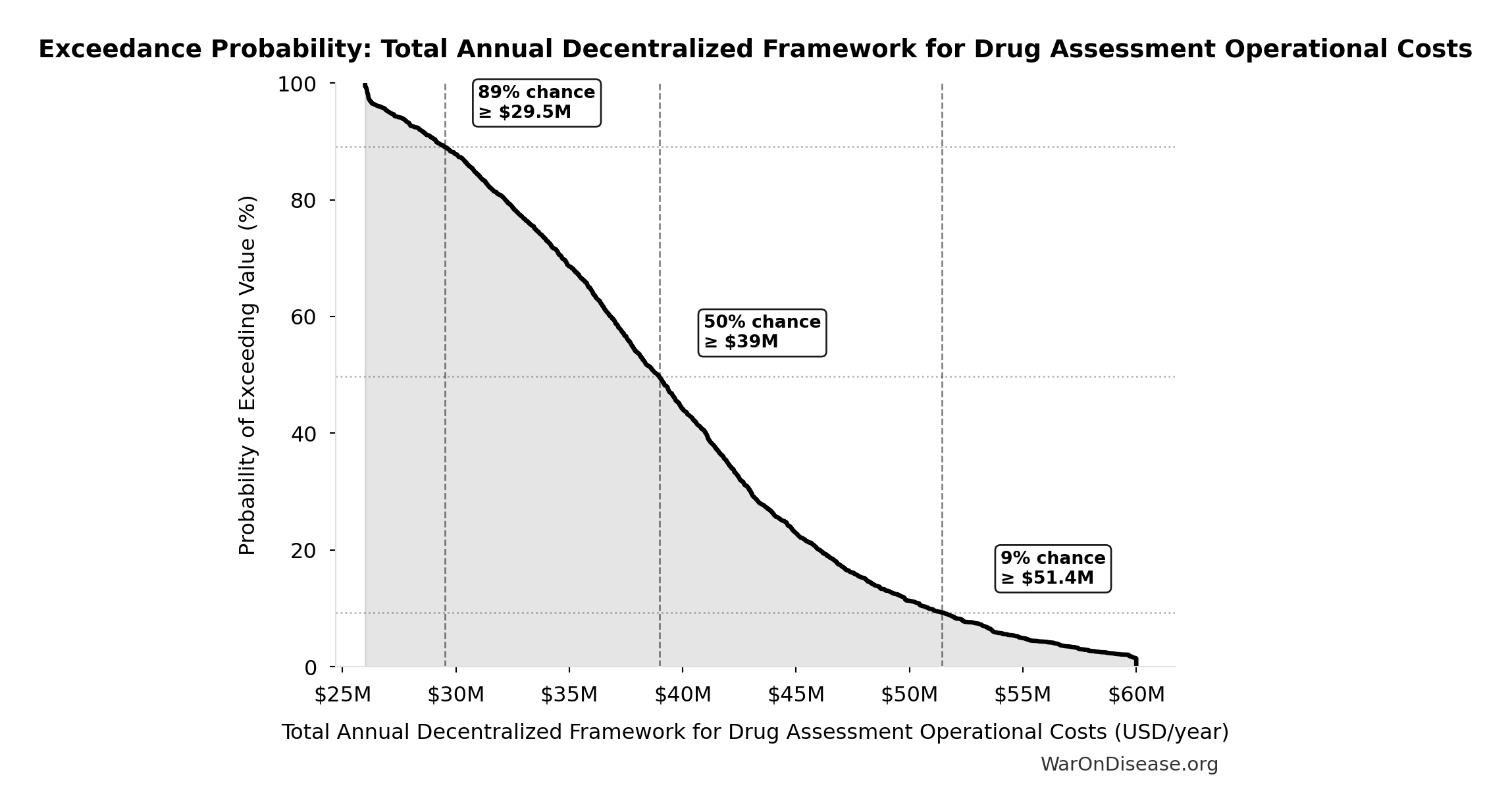
| Median (50th percentile) | $39M |
| Standard Deviation | $8.21M |
| 90% Range (5th-95th percentile) | [$27.3M, $55.6M] |
The histogram shows the distribution of Total Annual Decentralized Framework for Drug Assessment Operational Costs across 10,000 Monte Carlo simulations. The CDF (right) shows the probability of the outcome exceeding any given value, which is useful for risk assessment.
Exceedance Probability
This exceedance probability chart shows the likelihood that Total Annual Decentralized Framework for Drug Assessment Operational Costs will exceed any given threshold. Higher curves indicate more favorable outcomes with greater certainty.
Maximum Trial Capacity Multiplier (Physical Limit): 566x
Note📊 Details
Physical upper bound on trial-capacity multiplier from participant availability. Even with unlimited funding, annual trial enrollment cannot exceed willing participant pool.
Inputs:
- Global Patients Willing to Participate in Clinical Trials 🔢: 1.08 billion people
- Annual Global Clinical Trial Participants 📊: 1.9 million patients/year (95% CI: 1.5 million patients/year - 2.3 million patients/year)
\[ \begin{gathered} k_{capacity,max} \\ = \frac{N_{willing}}{Slots_{curr}} \\ = \frac{1.08B}{1.9M} \\ = 566 \end{gathered} \] where: \[ \begin{gathered} N_{willing} \\ = N_{patients} \times Pct_{willing} \\ = 2.4B \times 44.8\% \\ = 1.08B \end{gathered} \] ~ Medium confidence
Sensitivity Analysis
Sensitivity Indices for Maximum Trial Capacity Multiplier (Physical Limit)
Regression-based sensitivity showing which inputs explain the most variance in the output.
| Input Parameter | Sensitivity Coefficient | Interpretation |
|---|---|---|
| Global Patients Willing to Participate in Clinical Trials (people) | 0.8980 | Strong driver |
| Annual Global Clinical Trial Participants (patients/year) | 0.0989 | Minimal effect |
Interpretation: Standardized coefficients show the change in output (in SD units) per 1 SD change in input. Values near ±1 indicate strong influence; values exceeding ±1 may occur with correlated inputs.
Monte Carlo Distribution
Simulation Results Summary: Maximum Trial Capacity Multiplier (Physical Limit)
| Statistic | Value |
|---|---|
| Baseline (deterministic) | 566x |
| Mean (expected value) | 567x |
| Median (50th percentile) | 567x |
| Standard Deviation | 18.4x |
| 90% Range (5th-95th percentile) | [534x, 597x] |
The histogram shows the distribution of Maximum Trial Capacity Multiplier (Physical Limit) across 10,000 Monte Carlo simulations. The CDF (right) shows the probability of the outcome exceeding any given value, which is useful for risk assessment.
Exceedance Probability
This exceedance probability chart shows the likelihood that Maximum Trial Capacity Multiplier (Physical Limit) will exceed any given threshold. Higher curves indicate more favorable outcomes with greater certainty.
dFDA Patients Fundable Annually: 23.4 million patients/year
Note📊 Details
Number of patients fundable annually from dFDA funding at pragmatic trial cost. Source-agnostic counterpart of DIH_PATIENTS_FUNDABLE_ANNUALLY.
Inputs:
- dFDA Annual Trial Subsidies 🔢: $21.8B
- dFDA Pragmatic Trial Cost per Patient 📊: $929 (95% CI: $97 - $3K)
\[ \begin{gathered} N_{fundable,dFDA} \\ = \frac{Subsidies_{dFDA,ann}}{Cost_{pragmatic,pt}} \\ = \frac{\$21.8B}{\$929} \\ = 23.4M \end{gathered} \] where: \[ \begin{gathered} Subsidies_{dFDA,ann} \\ = Funding_{dFDA,ann} - OPEX_{dFDA} \\ = \$21.8B - \$40M \\ = \$21.8B \end{gathered} \] where: \[ \begin{gathered} OPEX_{dFDA} \\ = Cost_{platform} + Cost_{staff} + Cost_{infra} \\ + Cost_{regulatory} + Cost_{community} \\ = \$15M + \$10M + \$8M + \$5M + \$2M \\ = \$40M \end{gathered} \] ✓ High confidence
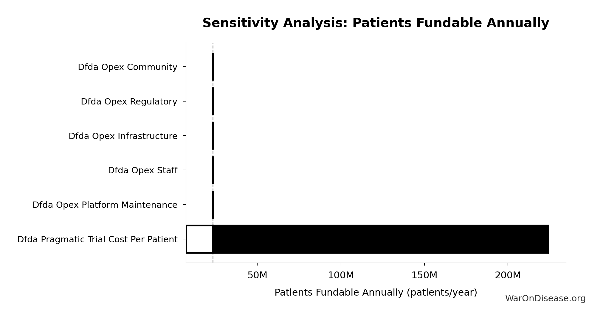
Sensitivity Analysis
Sensitivity Indices for dFDA Patients Fundable Annually
Regression-based sensitivity showing which inputs explain the most variance in the output.
| Input Parameter | Sensitivity Coefficient | Interpretation |
|---|---|---|
| dFDA Annual Trial Subsidies (USD/year) | 2.3351 | Strong driver |
| dFDA Pragmatic Trial Cost per Patient (USD/patient) | 1.5755 | Strong driver |
Interpretation: Standardized coefficients show the change in output (in SD units) per 1 SD change in input. Values near ±1 indicate strong influence; values exceeding ±1 may occur with correlated inputs.
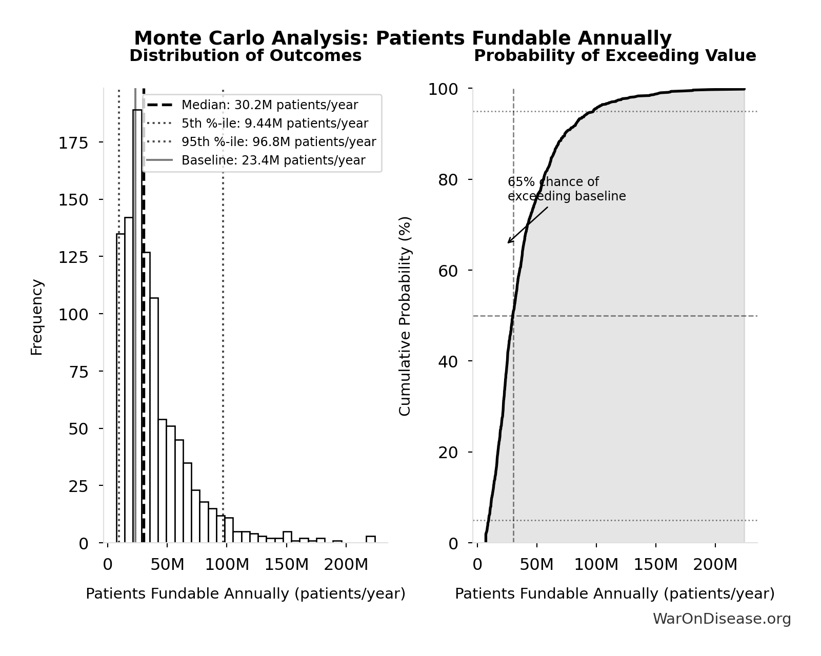
Monte Carlo Distribution
Simulation Results Summary: dFDA Patients Fundable Annually
| Statistic | Value |
|---|---|
| Baseline (deterministic) | 23.4 million |
| Mean (expected value) | 38.6 million |
| Median (50th percentile) | 30.2 million |
| Standard Deviation | 30.2 million |
| 90% Range (5th-95th percentile) | [9.46 million, 97 million] |
The histogram shows the distribution of dFDA Patients Fundable Annually across 10,000 Monte Carlo simulations. The CDF (right) shows the probability of the outcome exceeding any given value, which is useful for risk assessment.
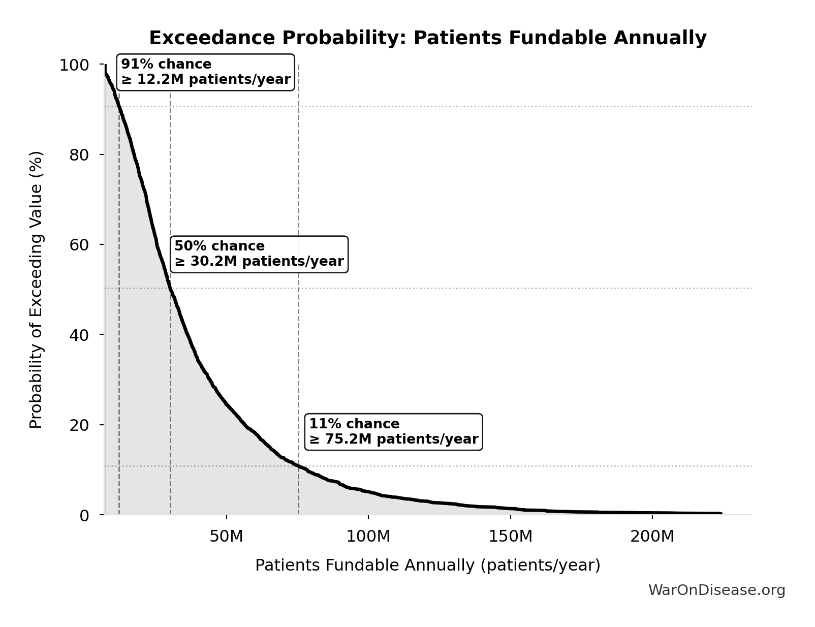
Exceedance Probability
This exceedance probability chart shows the likelihood that dFDA Patients Fundable Annually will exceed any given threshold. Higher curves indicate more favorable outcomes with greater certainty.
Trial Capacity Multiplier: 12.3x
Note📊 Details
Trial capacity multiplier from dFDA funding capacity vs. current global trial participation
Inputs:
- Annual Global Clinical Trial Participants 📊: 1.9 million patients/year (95% CI: 1.5 million patients/year - 2.3 million patients/year)
- dFDA Patients Fundable Annually 🔢: 23.4 million patients/year
\[ \begin{gathered} k_{capacity} \\ = \frac{N_{fundable,dFDA}}{Slots_{curr}} \\ = \frac{23.4M}{1.9M} \\ = 12.3 \end{gathered} \] where: \[ \begin{gathered} N_{fundable,dFDA} \\ = \frac{Subsidies_{dFDA,ann}}{Cost_{pragmatic,pt}} \\ = \frac{\$21.8B}{\$929} \\ = 23.4M \end{gathered} \] where: \[ \begin{gathered} Subsidies_{dFDA,ann} \\ = Funding_{dFDA,ann} - OPEX_{dFDA} \\ = \$21.8B - \$40M \\ = \$21.8B \end{gathered} \] where: \[ \begin{gathered} OPEX_{dFDA} \\ = Cost_{platform} + Cost_{staff} + Cost_{infra} \\ + Cost_{regulatory} + Cost_{community} \\ = \$15M + \$10M + \$8M + \$5M + \$2M \\ = \$40M \end{gathered} \] ✓ High confidence
Sensitivity Analysis
Sensitivity Indices for Trial Capacity Multiplier
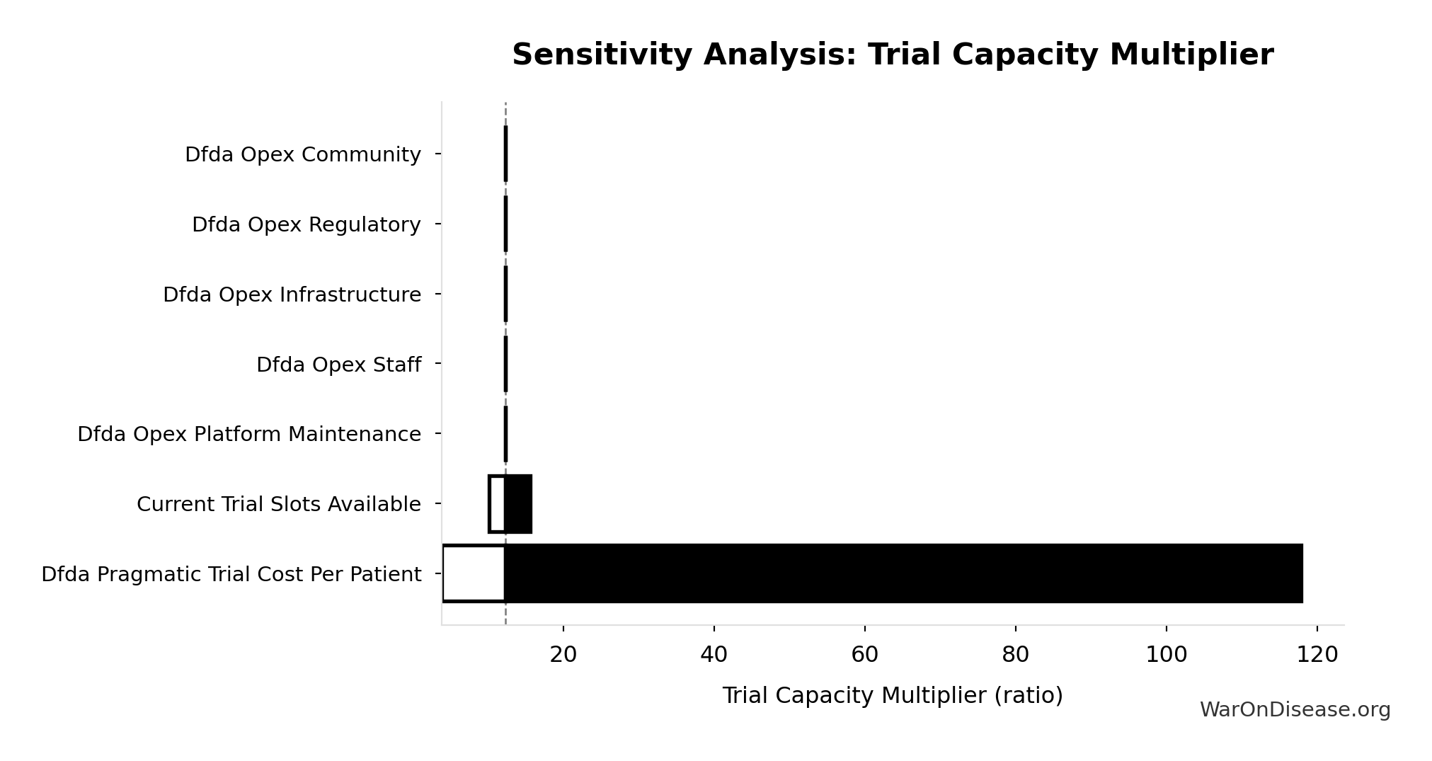
Regression-based sensitivity showing which inputs explain the most variance in the output.
| Input Parameter | Sensitivity Coefficient | Interpretation |
|---|---|---|
| dFDA Patients Fundable Annually (patients/year) | 1.0768 | Strong driver |
| Annual Global Clinical Trial Participants (patients/year) | 0.0910 | Minimal effect |
Interpretation: Standardized coefficients show the change in output (in SD units) per 1 SD change in input. Values near ±1 indicate strong influence; values exceeding ±1 may occur with correlated inputs.
Monte Carlo Distribution
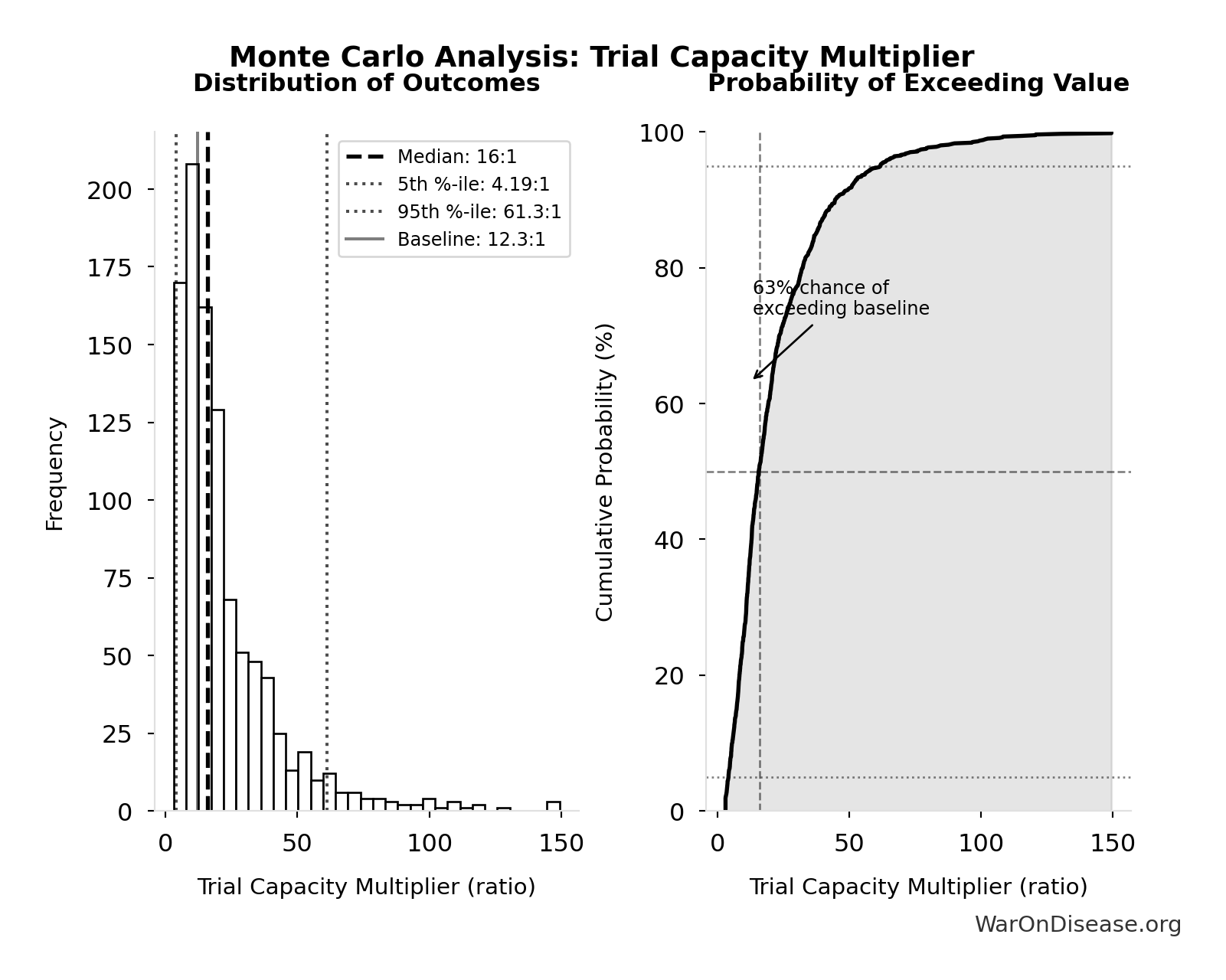
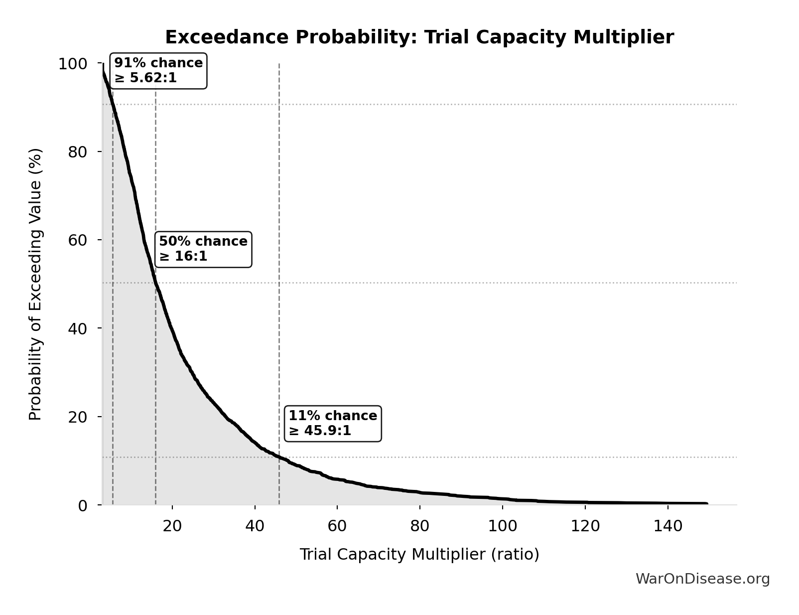
Simulation Results Summary: Trial Capacity Multiplier
| Statistic | Value |
|---|---|
| Baseline (deterministic) | 12.3x |
| Mean (expected value) | 22.1x |
| Median (50th percentile) | 16x |
| Standard Deviation | 20.2x |
| 90% Range (5th-95th percentile) | [4.2x, 61.4x] |
The histogram shows the distribution of Trial Capacity Multiplier across 10,000 Monte Carlo simulations. The CDF (right) shows the probability of the outcome exceeding any given value, which is useful for risk assessment.
Exceedance Probability
This exceedance probability chart shows the likelihood that Trial Capacity Multiplier will exceed any given threshold. Higher curves indicate more favorable outcomes with greater certainty.
Total DALYs from Elimination of Efficacy Lag Plus Earlier Treatment Discovery from Higher Trial Throughput: 565 billion DALYs
Note📊 Details
Total DALYs averted from the combined dFDA timeline shift. Calculated as annual global DALY burden × eventually avoidable percentage × timeline shift years. Includes both fatal and non-fatal diseases (WHO GBD methodology).
Inputs:
- Global Annual DALY Burden 📊: 2.88 billion DALYs/year (SE: ±150 million DALYs/year)
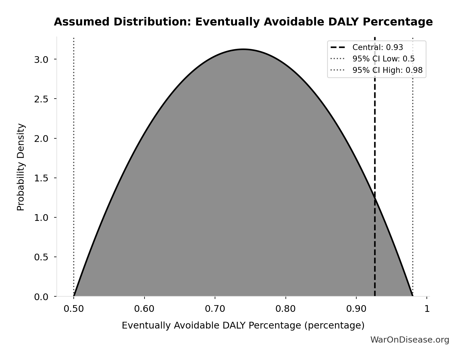
- Eventually Avoidable DALY Percentage: 92.6% (95% CI: 50% - 98%)
- dFDA Average Total Timeline Shift 🔢: 212 years
\[ \begin{gathered} DALYs_{max} \\ = DALYs_{global,ann} \times Pct_{avoid,DALY} \times T_{accel,max} \\ = 2.88B \times 92.6\% \times 212 \\ = 565B \end{gathered} \] where: \[ T_{accel,max} = T_{accel} + T_{lag} = 204 + 8.2 = 212 \] where: \[ \begin{gathered} T_{accel} \\ = T_{first,SQ} \times \left(1 - \frac{1}{k_{capacity}}\right) \\ = 222 \times \left(1 - \frac{1}{12.3}\right) \\ = 204 \end{gathered} \] where: \[ \begin{gathered} T_{first,SQ} \\ = T_{queue,SQ} \times 0.5 \\ = 443 \times 0.5 \\ = 222 \end{gathered} \] where: \[ \begin{gathered} T_{queue,SQ} \\ = \frac{N_{untreated}}{Treatments_{new,ann}} \\ = \frac{6{,}650}{15} \\ = 443 \end{gathered} \] where: \[ \begin{gathered} N_{untreated} \\ = N_{rare} \times 0.95 \\ = 7{,}000 \times 0.95 \\ = 6{,}650 \end{gathered} \] where: \[ \begin{gathered} k_{capacity} \\ = \frac{N_{fundable,dFDA}}{Slots_{curr}} \\ = \frac{23.4M}{1.9M} \\ = 12.3 \end{gathered} \] where: \[ \begin{gathered} N_{fundable,dFDA} \\ = \frac{Subsidies_{dFDA,ann}}{Cost_{pragmatic,pt}} \\ = \frac{\$21.8B}{\$929} \\ = 23.4M \end{gathered} \] where: \[ \begin{gathered} Subsidies_{dFDA,ann} \\ = Funding_{dFDA,ann} - OPEX_{dFDA} \\ = \$21.8B - \$40M \\ = \$21.8B \end{gathered} \] where: \[ \begin{gathered} OPEX_{dFDA} \\ = Cost_{platform} + Cost_{staff} + Cost_{infra} \\ + Cost_{regulatory} + Cost_{community} \\ = \$15M + \$10M + \$8M + \$5M + \$2M \\ = \$40M \end{gathered} \] ? Low confidence
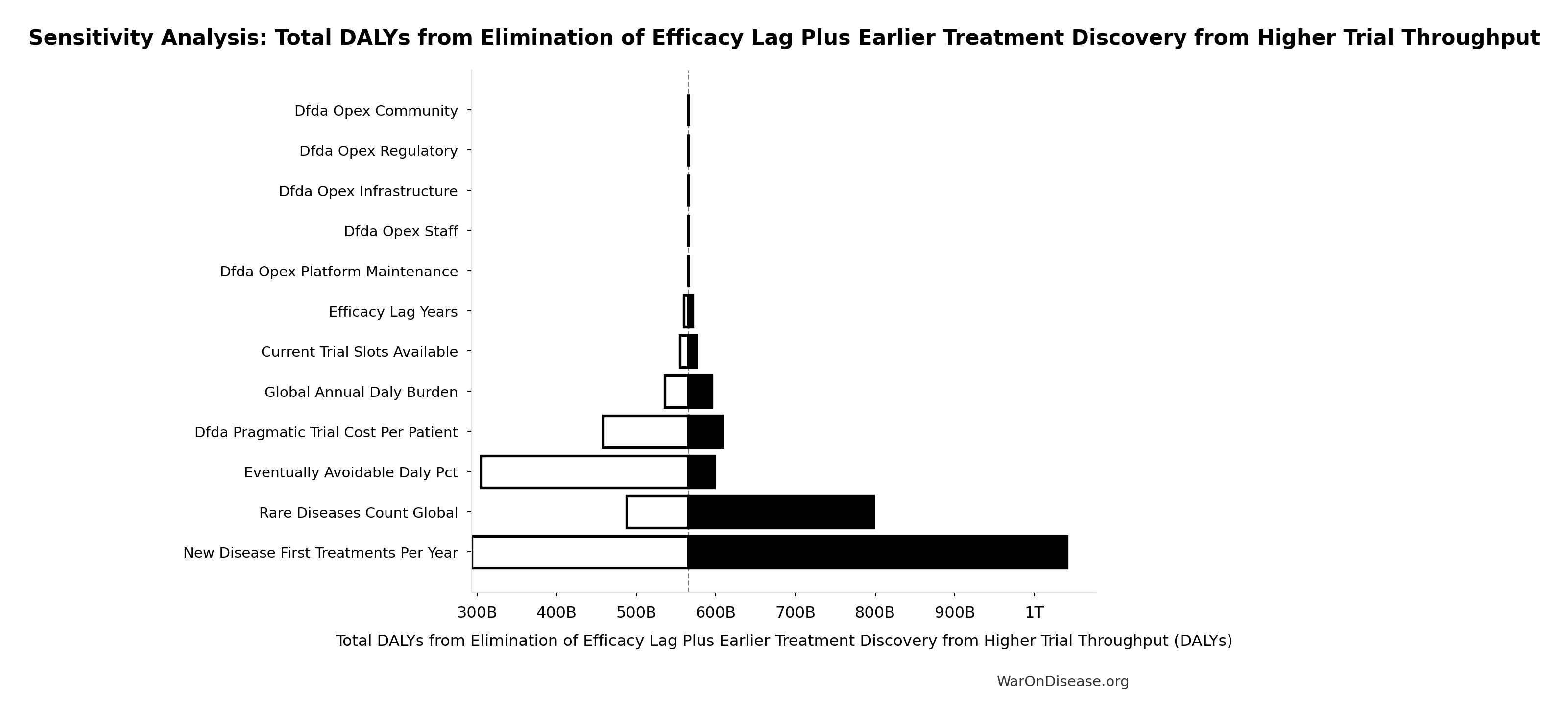
Sensitivity Analysis
Sensitivity Indices for Total DALYs from Elimination of Efficacy Lag Plus Earlier Treatment Discovery from Higher Trial Throughput
Regression-based sensitivity showing which inputs explain the most variance in the output.
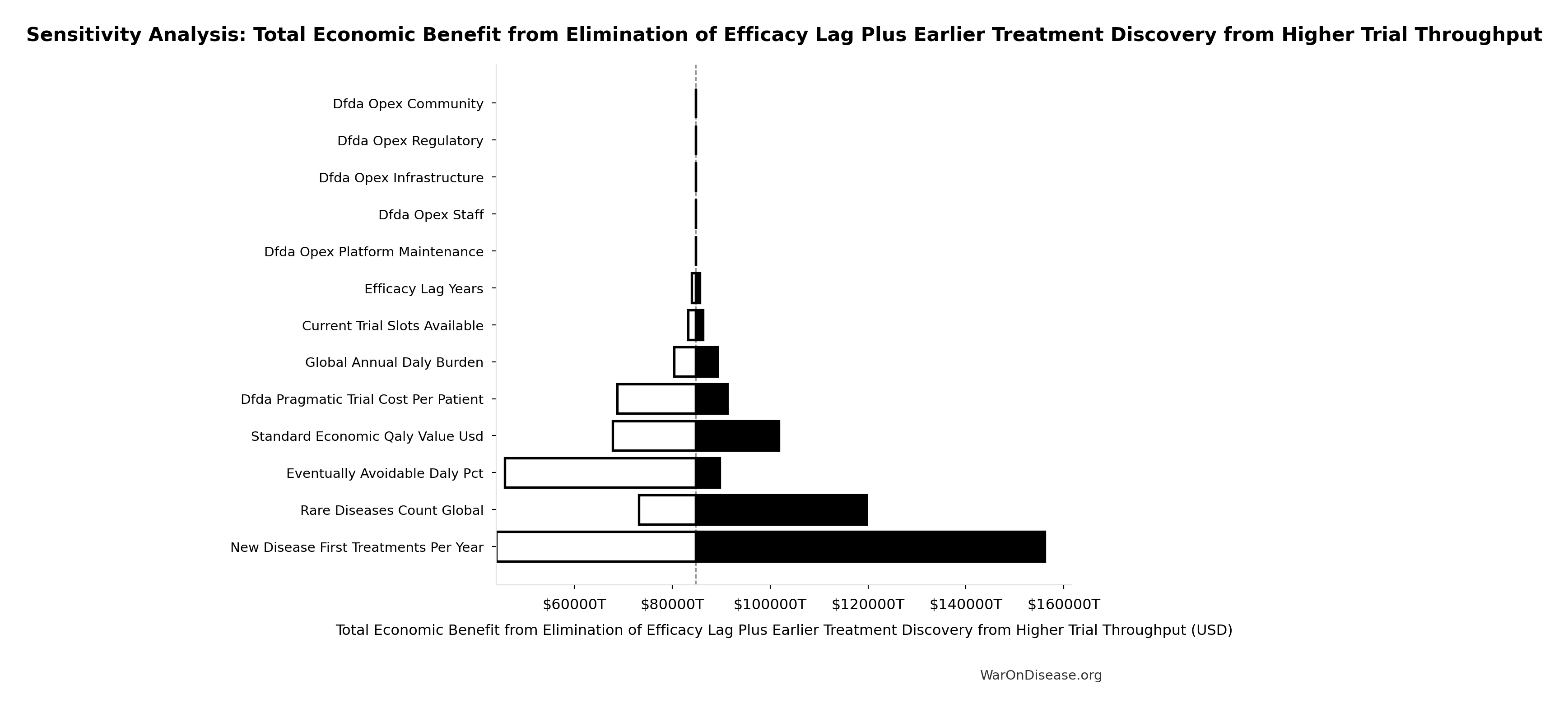
| Input Parameter | Sensitivity Coefficient | Interpretation |
|---|---|---|
| dFDA Average Total Timeline Shift (years) | 0.8999 | Strong driver |
| Eventually Avoidable DALY Percentage (percentage) | 0.4866 | Moderate driver |
| Global Annual DALY Burden (DALYs/year) | 0.0432 | Minimal effect |
Interpretation: Standardized coefficients show the change in output (in SD units) per 1 SD change in input. Values near ±1 indicate strong influence; values exceeding ±1 may occur with correlated inputs.
Monte Carlo Distribution
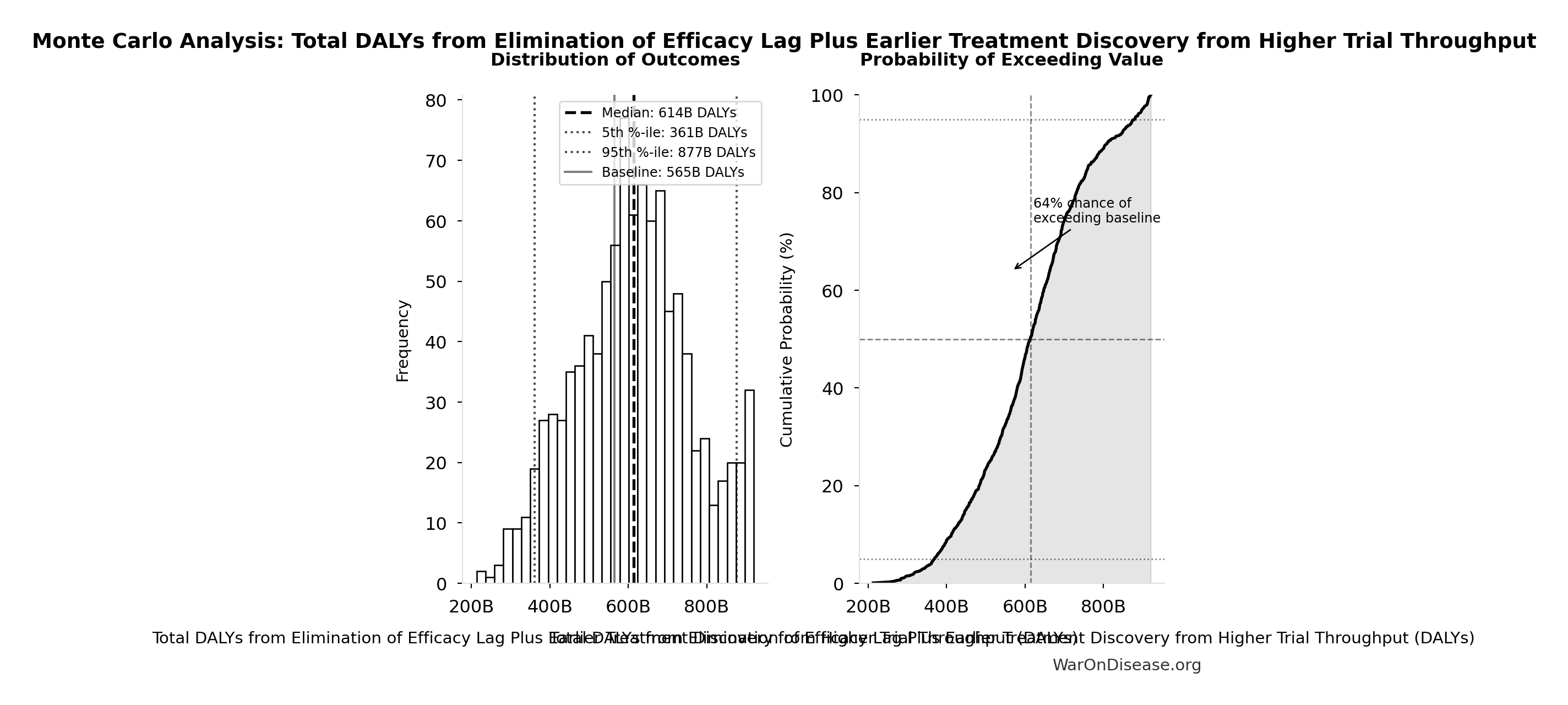
Simulation Results Summary: Total DALYs from Elimination of Efficacy Lag Plus Earlier Treatment Discovery from Higher Trial Throughput
| Statistic | Value |
|---|---|
| Baseline (deterministic) | 565 billion |
| Mean (expected value) | 610 billion |
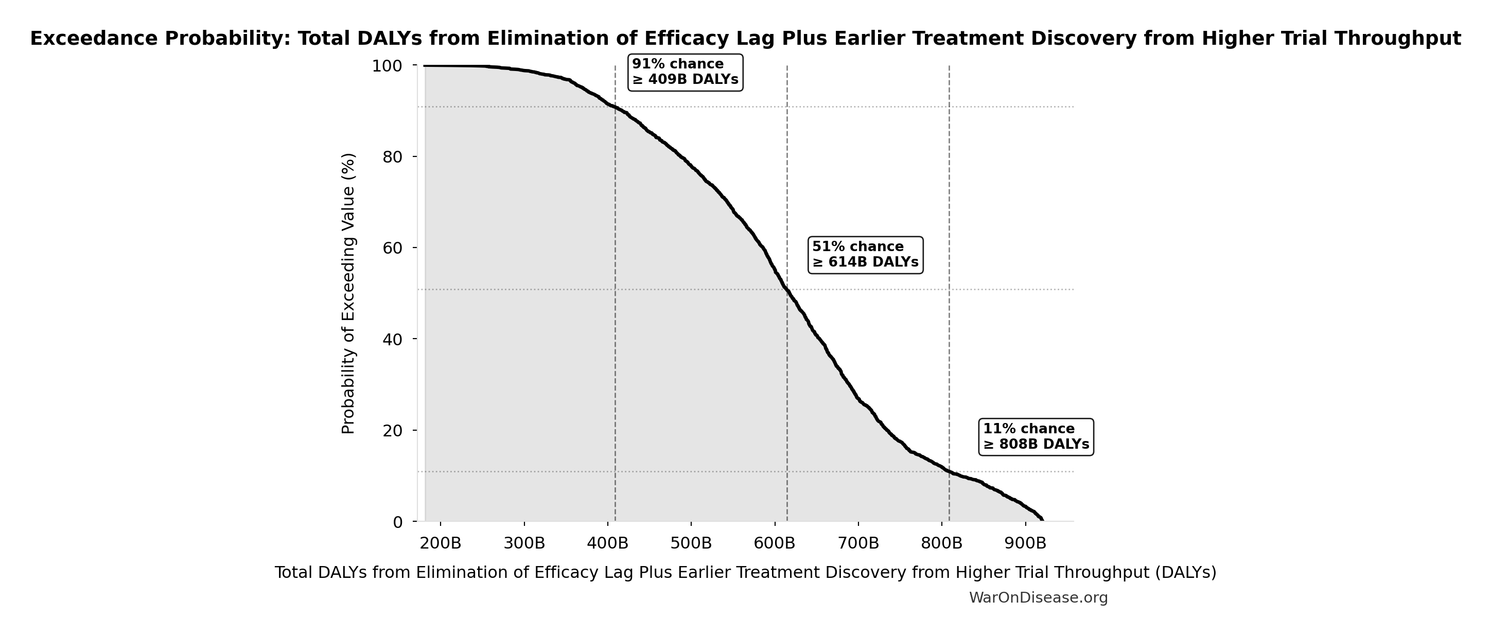
| Median (50th percentile) | 614 billion |
| Standard Deviation | 148 billion |
| 90% Range (5th-95th percentile) | [361 billion, 877 billion] |
The histogram shows the distribution of Total DALYs from Elimination of Efficacy Lag Plus Earlier Treatment Discovery from Higher Trial Throughput across 10,000 Monte Carlo simulations. The CDF (right) shows the probability of the outcome exceeding any given value, which is useful for risk assessment.
Exceedance Probability
This exceedance probability chart shows the likelihood that Total DALYs from Elimination of Efficacy Lag Plus Earlier Treatment Discovery from Higher Trial Throughput will exceed any given threshold. Higher curves indicate more favorable outcomes with greater certainty.
Total Economic Benefit from Elimination of Efficacy Lag Plus Earlier Treatment Discovery from Higher Trial Throughput: $84.8 quadrillion
Note📊 Details
Total economic value from the combined dFDA timeline shift. DALYs valued at standard economic rate.
Inputs:
- Total DALYs from Elimination of Efficacy Lag Plus Earlier Treatment Discovery from Higher Trial Throughput 🔢: 565 billion DALYs
- Standard Economic Value per QALY 📊: $150K (SE: ±$30K)
\[ \begin{gathered} Value_{max} \\ = DALYs_{max} \times Value_{QALY} \\ = 565B \times \$150K \\ = \$84800T \end{gathered} \] where: \[ \begin{gathered} DALYs_{max} \\ = DALYs_{global,ann} \times Pct_{avoid,DALY} \times T_{accel,max} \\ = 2.88B \times 92.6\% \times 212 \\ = 565B \end{gathered} \] where: \[ T_{accel,max} = T_{accel} + T_{lag} = 204 + 8.2 = 212 \] where: \[ \begin{gathered} T_{accel} \\ = T_{first,SQ} \times \left(1 - \frac{1}{k_{capacity}}\right) \\ = 222 \times \left(1 - \frac{1}{12.3}\right) \\ = 204 \end{gathered} \] where: \[ \begin{gathered} T_{first,SQ} \\ = T_{queue,SQ} \times 0.5 \\ = 443 \times 0.5 \\ = 222 \end{gathered} \] where: \[ \begin{gathered} T_{queue,SQ} \\ = \frac{N_{untreated}}{Treatments_{new,ann}} \\ = \frac{6{,}650}{15} \\ = 443 \end{gathered} \] where: \[ \begin{gathered} N_{untreated} \\ = N_{rare} \times 0.95 \\ = 7{,}000 \times 0.95 \\ = 6{,}650 \end{gathered} \] where: \[ \begin{gathered} k_{capacity} \\ = \frac{N_{fundable,dFDA}}{Slots_{curr}} \\ = \frac{23.4M}{1.9M} \\ = 12.3 \end{gathered} \] where: \[ \begin{gathered} N_{fundable,dFDA} \\ = \frac{Subsidies_{dFDA,ann}}{Cost_{pragmatic,pt}} \\ = \frac{\$21.8B}{\$929} \\ = 23.4M \end{gathered} \] where: \[ \begin{gathered} Subsidies_{dFDA,ann} \\ = Funding_{dFDA,ann} - OPEX_{dFDA} \\ = \$21.8B - \$40M \\ = \$21.8B \end{gathered} \] where: \[ \begin{gathered} OPEX_{dFDA} \\ = Cost_{platform} + Cost_{staff} + Cost_{infra} \\ + Cost_{regulatory} + Cost_{community} \\ = \$15M + \$10M + \$8M + \$5M + \$2M \\ = \$40M \end{gathered} \] ? Low confidence
Sensitivity Analysis
Sensitivity Indices for Total Economic Benefit from Elimination of Efficacy Lag Plus Earlier Treatment Discovery from Higher Trial Throughput
Regression-based sensitivity showing which inputs explain the most variance in the output.
| Input Parameter | Sensitivity Coefficient | Interpretation |
|---|---|---|
| Total DALYs from Elimination of Efficacy Lag Plus Earlier Treatment Discovery from Higher Trial Throughput (DALYs) | 1.7788 | Strong driver |
| Standard Economic Value per QALY (USD/QALY) | 1.3381 | Strong driver |
Interpretation: Standardized coefficients show the change in output (in SD units) per 1 SD change in input. Values near ±1 indicate strong influence; values exceeding ±1 may occur with correlated inputs.
Monte Carlo Distribution
Simulation Results Summary: Total Economic Benefit from Elimination of Efficacy Lag Plus Earlier Treatment Discovery from Higher Trial Throughput
| Statistic | Value |
|---|---|
| Baseline (deterministic) | $84.8 quadrillion |
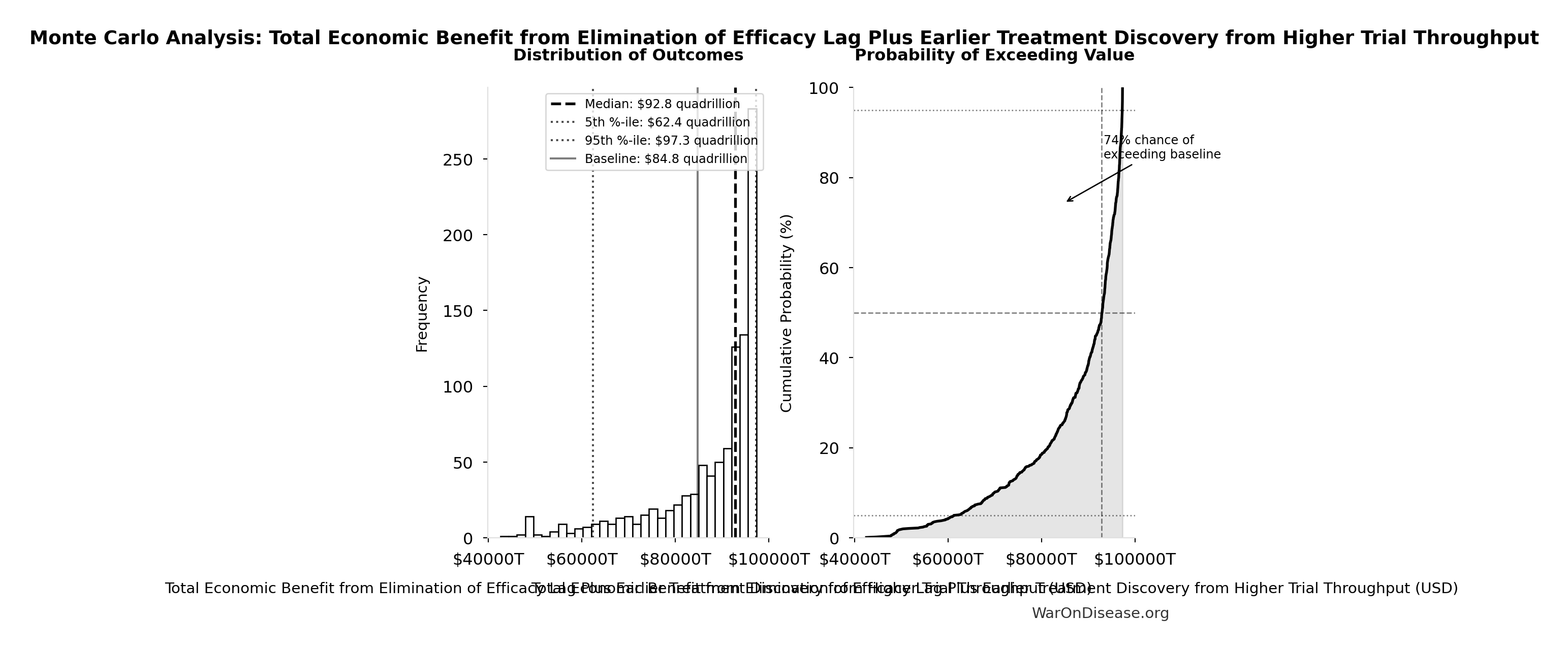
| Mean (expected value) | $87.8 quadrillion |
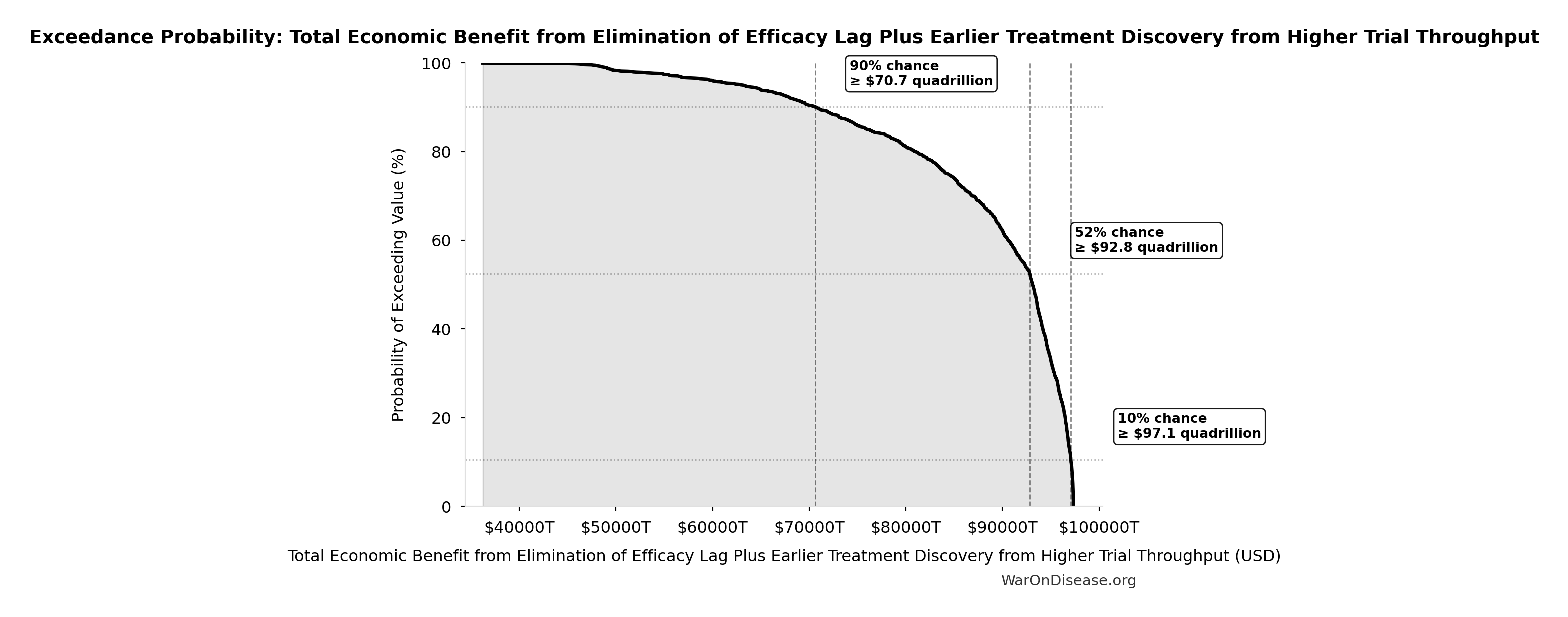
| Median (50th percentile) | $92.9 quadrillion |
| Standard Deviation | $11.5 quadrillion |
| 90% Range (5th-95th percentile) | [$62.4 quadrillion, $97.3 quadrillion] |
The histogram shows the distribution of Total Economic Benefit from Elimination of Efficacy Lag Plus Earlier Treatment Discovery from Higher Trial Throughput across 10,000 Monte Carlo simulations. The CDF (right) shows the probability of the outcome exceeding any given value, which is useful for risk assessment.
Exceedance Probability
This exceedance probability chart shows the likelihood that Total Economic Benefit from Elimination of Efficacy Lag Plus Earlier Treatment Discovery from Higher Trial Throughput will exceed any given threshold. Higher curves indicate more favorable outcomes with greater certainty.
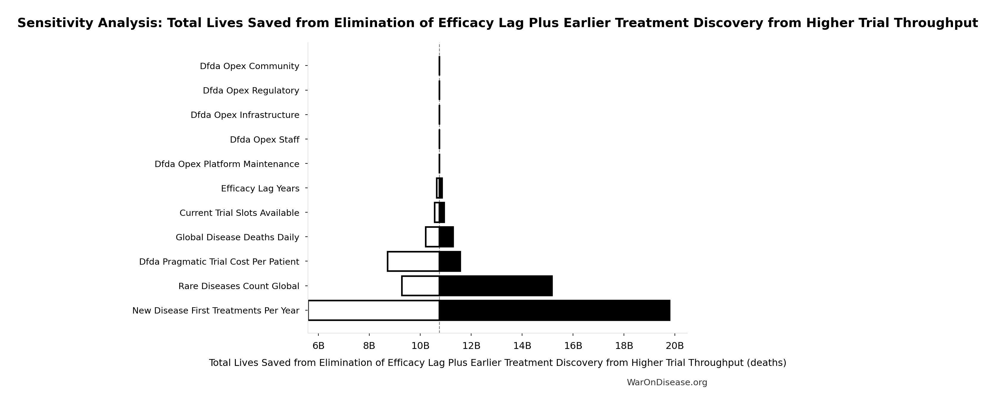
Total Lives Saved from Elimination of Efficacy Lag Plus Earlier Treatment Discovery from Higher Trial Throughput: 10.7 billion deaths
Note📊 Details
Total eventually avoidable deaths from the combined dFDA timeline shift. Represents deaths prevented when cures arrive earlier due to both increased trial capacity and eliminated efficacy lag.
Inputs:
- Global Daily Deaths from Disease and Aging 📊: 150 thousand deaths/day (SE: ±7.5 thousand deaths/day)
- dFDA Average Total Timeline Shift 🔢: 212 years
\[ \begin{gathered} Lives_{max} \\ = Deaths_{disease,daily} \times T_{accel,max} \times 338 \\ = 150{,}000 \times 212 \times 338 \\ = 10.7B \end{gathered} \] where: \[ T_{accel,max} = T_{accel} + T_{lag} = 204 + 8.2 = 212 \] where: \[ \begin{gathered} T_{accel} \\ = T_{first,SQ} \times \left(1 - \frac{1}{k_{capacity}}\right) \\ = 222 \times \left(1 - \frac{1}{12.3}\right) \\ = 204 \end{gathered} \] where: \[ \begin{gathered} T_{first,SQ} \\ = T_{queue,SQ} \times 0.5 \\ = 443 \times 0.5 \\ = 222 \end{gathered} \] where: \[ \begin{gathered} T_{queue,SQ} \\ = \frac{N_{untreated}}{Treatments_{new,ann}} \\ = \frac{6{,}650}{15} \\ = 443 \end{gathered} \] where: \[ \begin{gathered} N_{untreated} \\ = N_{rare} \times 0.95 \\ = 7{,}000 \times 0.95 \\ = 6{,}650 \end{gathered} \] where: \[ \begin{gathered} k_{capacity} \\ = \frac{N_{fundable,dFDA}}{Slots_{curr}} \\ = \frac{23.4M}{1.9M} \\ = 12.3 \end{gathered} \] where: \[ \begin{gathered} N_{fundable,dFDA} \\ = \frac{Subsidies_{dFDA,ann}}{Cost_{pragmatic,pt}} \\ = \frac{\$21.8B}{\$929} \\ = 23.4M \end{gathered} \] where: \[ \begin{gathered} Subsidies_{dFDA,ann} \\ = Funding_{dFDA,ann} - OPEX_{dFDA} \\ = \$21.8B - \$40M \\ = \$21.8B \end{gathered} \] where: \[ \begin{gathered} OPEX_{dFDA} \\ = Cost_{platform} + Cost_{staff} + Cost_{infra} \\ + Cost_{regulatory} + Cost_{community} \\ = \$15M + \$10M + \$8M + \$5M + \$2M \\ = \$40M \end{gathered} \] ? Low confidence
Sensitivity Analysis
Sensitivity Indices for Total Lives Saved from Elimination of Efficacy Lag Plus Earlier Treatment Discovery from Higher Trial Throughput
Regression-based sensitivity showing which inputs explain the most variance in the output.
| Input Parameter | Sensitivity Coefficient | Interpretation |
|---|---|---|
| dFDA Average Total Timeline Shift (years) | 1.0374 | Strong driver |
| Global Daily Deaths from Disease and Aging (deaths/day) | 0.0406 | Minimal effect |
Interpretation: Standardized coefficients show the change in output (in SD units) per 1 SD change in input. Values near ±1 indicate strong influence; values exceeding ±1 may occur with correlated inputs.
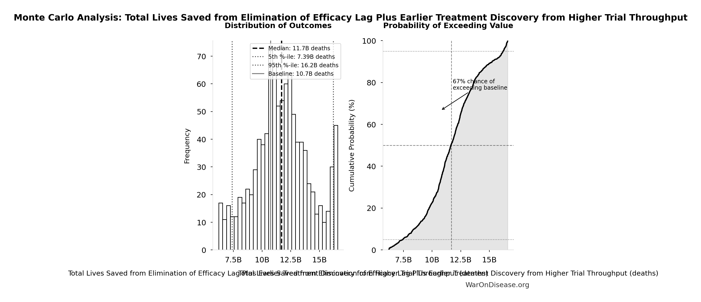
Monte Carlo Distribution
Simulation Results Summary: Total Lives Saved from Elimination of Efficacy Lag Plus Earlier Treatment Discovery from Higher Trial Throughput
| Statistic | Value |
|---|---|
| Baseline (deterministic) | 10.7 billion |
| Mean (expected value) | 11.7 billion |
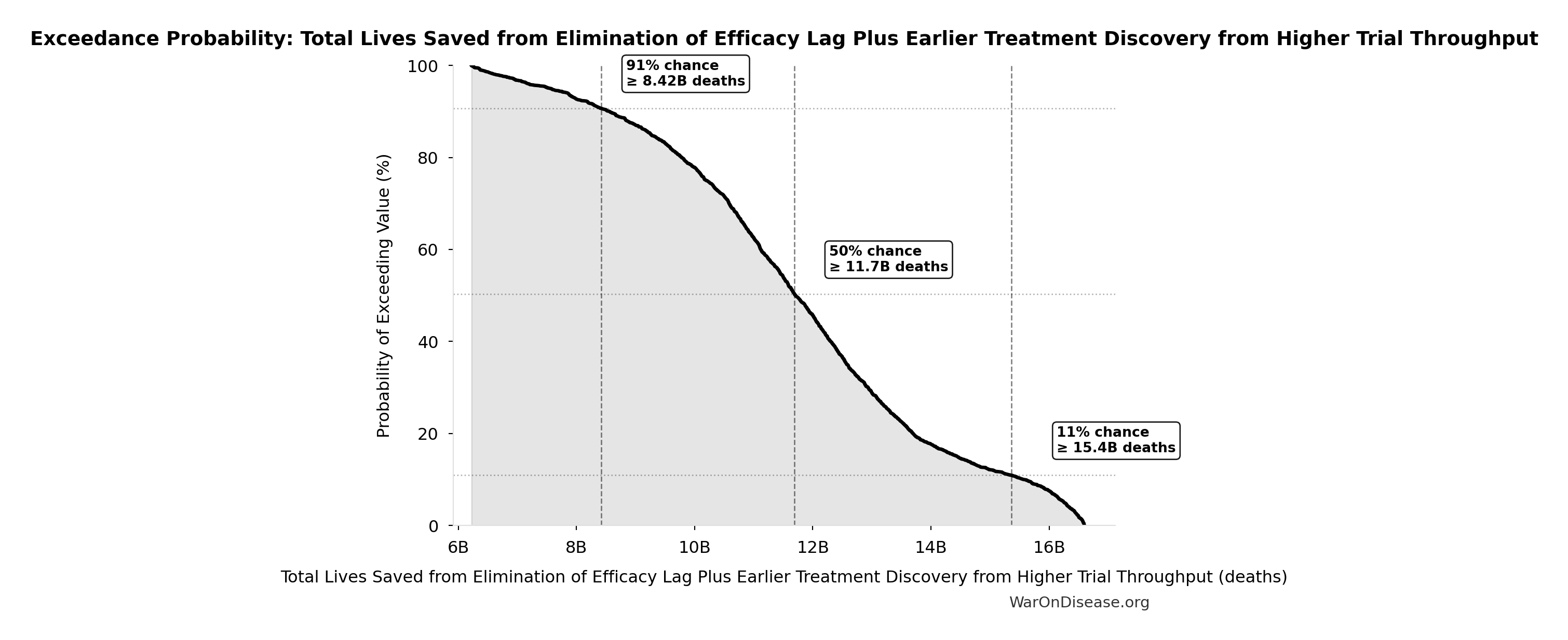
| Median (50th percentile) | 11.7 billion |
| Standard Deviation | 2.45 billion |
| 90% Range (5th-95th percentile) | [7.4 billion, 16.2 billion] |
The histogram shows the distribution of Total Lives Saved from Elimination of Efficacy Lag Plus Earlier Treatment Discovery from Higher Trial Throughput across 10,000 Monte Carlo simulations. The CDF (right) shows the probability of the outcome exceeding any given value, which is useful for risk assessment.
Exceedance Probability
This exceedance probability chart shows the likelihood that Total Lives Saved from Elimination of Efficacy Lag Plus Earlier Treatment Discovery from Higher Trial Throughput will exceed any given threshold. Higher curves indicate more favorable outcomes with greater certainty.
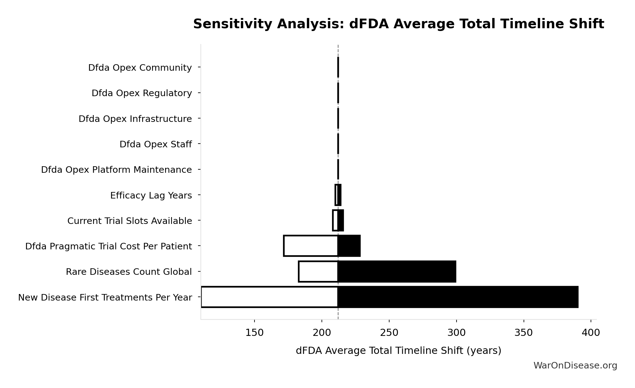
dFDA Average Total Timeline Shift: 212 years
Note📊 Details
Average years earlier patients receive treatments due to dFDA. Combines treatment timeline acceleration from increased trial capacity with efficacy lag elimination for treatments already discovered.
Inputs:
- dFDA Treatment Timeline Acceleration 🔢: 204 years
- Regulatory Delay for Efficacy Testing Post-Safety Verification 📊: 8.2 years (SE: ±2 years)
\[ T_{accel,max} = T_{accel} + T_{lag} = 204 + 8.2 = 212 \] where: \[ \begin{gathered} T_{accel} \\ = T_{first,SQ} \times \left(1 - \frac{1}{k_{capacity}}\right) \\ = 222 \times \left(1 - \frac{1}{12.3}\right) \\ = 204 \end{gathered} \] where: \[ \begin{gathered} T_{first,SQ} \\ = T_{queue,SQ} \times 0.5 \\ = 443 \times 0.5 \\ = 222 \end{gathered} \] where: \[ \begin{gathered} T_{queue,SQ} \\ = \frac{N_{untreated}}{Treatments_{new,ann}} \\ = \frac{6{,}650}{15} \\ = 443 \end{gathered} \] where: \[ \begin{gathered} N_{untreated} \\ = N_{rare} \times 0.95 \\ = 7{,}000 \times 0.95 \\ = 6{,}650 \end{gathered} \] where: \[ \begin{gathered} k_{capacity} \\ = \frac{N_{fundable,dFDA}}{Slots_{curr}} \\ = \frac{23.4M}{1.9M} \\ = 12.3 \end{gathered} \] where: \[ \begin{gathered} N_{fundable,dFDA} \\ = \frac{Subsidies_{dFDA,ann}}{Cost_{pragmatic,pt}} \\ = \frac{\$21.8B}{\$929} \\ = 23.4M \end{gathered} \] where: \[ \begin{gathered} Subsidies_{dFDA,ann} \\ = Funding_{dFDA,ann} - OPEX_{dFDA} \\ = \$21.8B - \$40M \\ = \$21.8B \end{gathered} \] where: \[ \begin{gathered} OPEX_{dFDA} \\ = Cost_{platform} + Cost_{staff} + Cost_{infra} \\ + Cost_{regulatory} + Cost_{community} \\ = \$15M + \$10M + \$8M + \$5M + \$2M \\ = \$40M \end{gathered} \] ? Low confidence
Sensitivity Analysis

Sensitivity Indices for dFDA Average Total Timeline Shift
Regression-based sensitivity showing which inputs explain the most variance in the output.
| Input Parameter | Sensitivity Coefficient | Interpretation |
|---|---|---|
| dFDA Treatment Timeline Acceleration (years) | 1.0325 | Strong driver |
| Regulatory Delay for Efficacy Testing Post-Safety Verification (years) | 0.0328 | Minimal effect |
Interpretation: Standardized coefficients show the change in output (in SD units) per 1 SD change in input. Values near ±1 indicate strong influence; values exceeding ±1 may occur with correlated inputs.
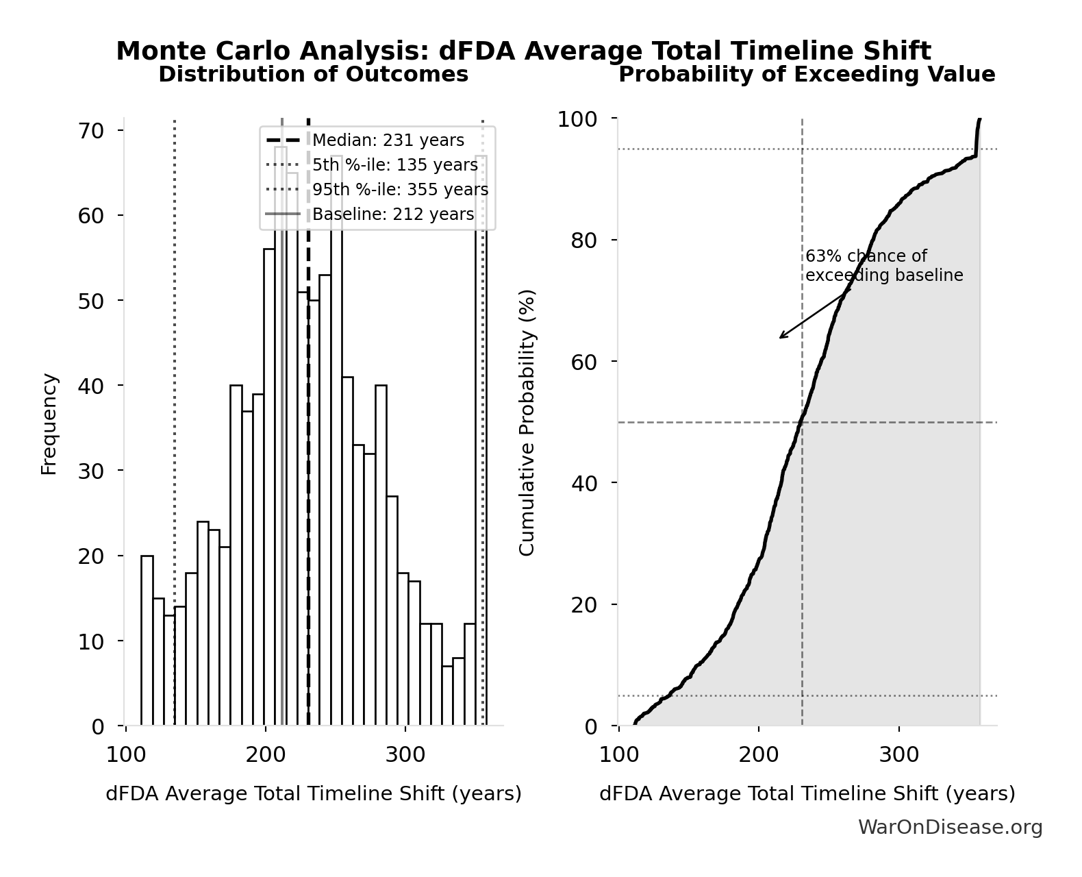
Monte Carlo Distribution
Simulation Results Summary: dFDA Average Total Timeline Shift
| Statistic | Value |
|---|---|
| Baseline (deterministic) | 212 |
| Mean (expected value) | 233 |
| Median (50th percentile) | 231 |
| Standard Deviation | 60.3 |
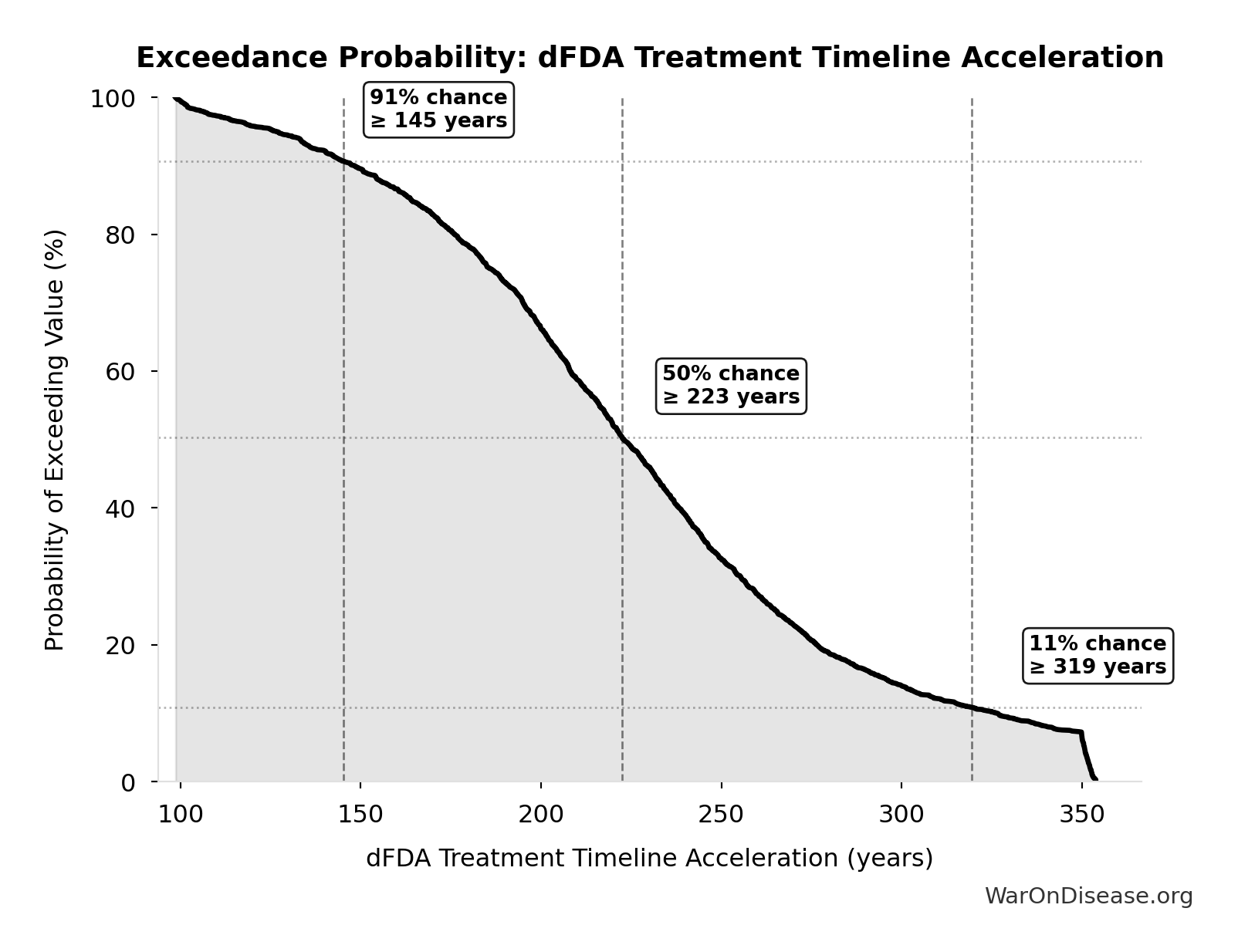
| 90% Range (5th-95th percentile) | [135, 355] |
The histogram shows the distribution of dFDA Average Total Timeline Shift across 10,000 Monte Carlo simulations. The CDF (right) shows the probability of the outcome exceeding any given value, which is useful for risk assessment.
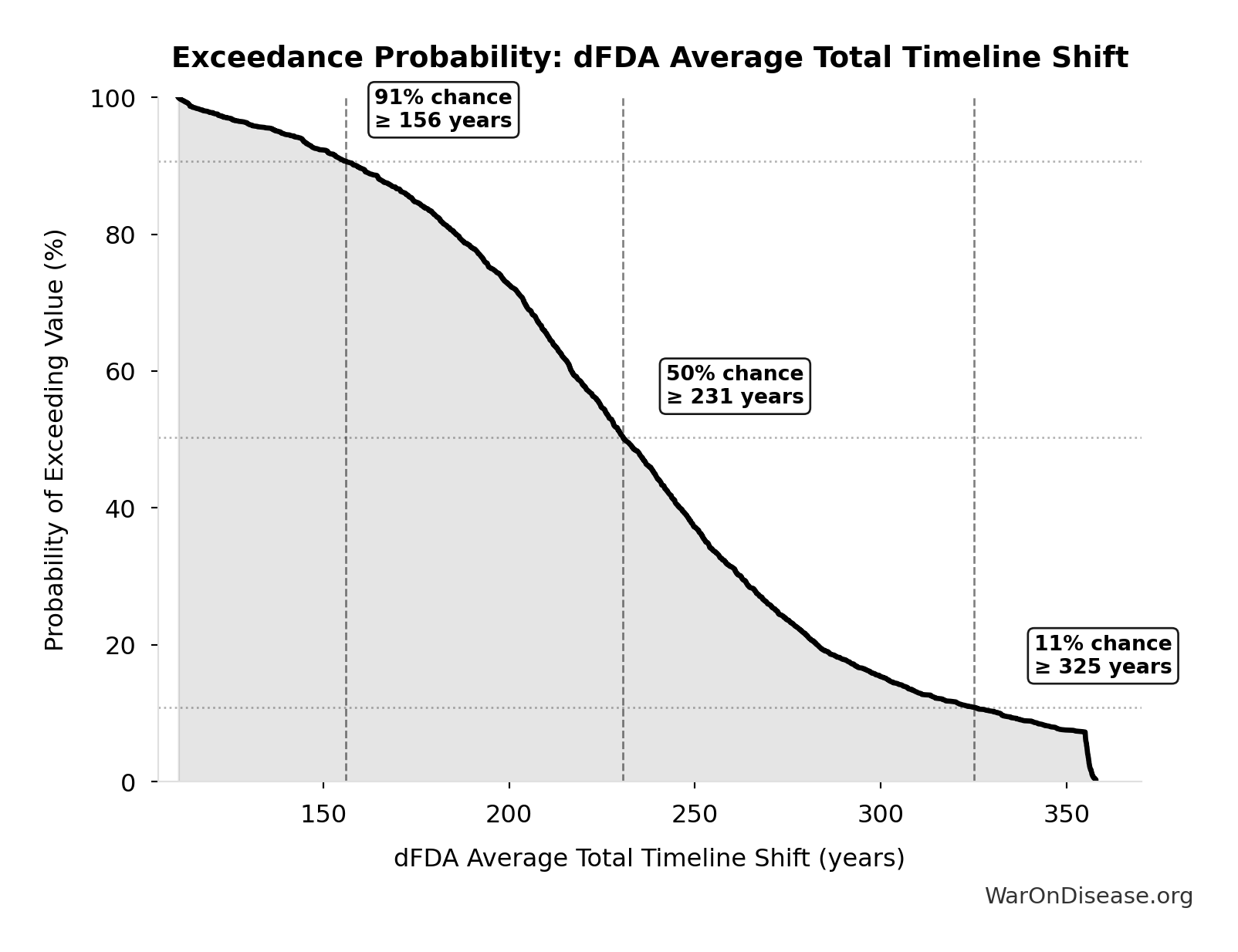
Exceedance Probability
This exceedance probability chart shows the likelihood that dFDA Average Total Timeline Shift will exceed any given threshold. Higher curves indicate more favorable outcomes with greater certainty.
dFDA Treatment Timeline Acceleration: 204 years
Note📊 Details
Years earlier the average first treatment arrives due to dFDA’s trial capacity increase. Calculated as the status quo timeline reduced by the inverse of the capacity multiplier. Uses only trial capacity multiplier (not combined with valley of death rescue) because additional candidates don’t directly speed therapeutic space exploration.
Inputs:
- Status Quo Average Years to First Treatment 🔢: 222 years
- Trial Capacity Multiplier 🔢: 12.3x
\[ \begin{gathered} T_{accel} \\ = T_{first,SQ} \times \left(1 - \frac{1}{k_{capacity}}\right) \\ = 222 \times \left(1 - \frac{1}{12.3}\right) \\ = 204 \end{gathered} \] where: \[ \begin{gathered} T_{first,SQ} \\ = T_{queue,SQ} \times 0.5 \\ = 443 \times 0.5 \\ = 222 \end{gathered} \] where: \[ \begin{gathered} T_{queue,SQ} \\ = \frac{N_{untreated}}{Treatments_{new,ann}} \\ = \frac{6{,}650}{15} \\ = 443 \end{gathered} \] where: \[ \begin{gathered} N_{untreated} \\ = N_{rare} \times 0.95 \\ = 7{,}000 \times 0.95 \\ = 6{,}650 \end{gathered} \] where: \[ \begin{gathered} k_{capacity} \\ = \frac{N_{fundable,dFDA}}{Slots_{curr}} \\ = \frac{23.4M}{1.9M} \\ = 12.3 \end{gathered} \] where: \[ \begin{gathered} N_{fundable,dFDA} \\ = \frac{Subsidies_{dFDA,ann}}{Cost_{pragmatic,pt}} \\ = \frac{\$21.8B}{\$929} \\ = 23.4M \end{gathered} \] where: \[ \begin{gathered} Subsidies_{dFDA,ann} \\ = Funding_{dFDA,ann} - OPEX_{dFDA} \\ = \$21.8B - \$40M \\ = \$21.8B \end{gathered} \] where: \[ \begin{gathered} OPEX_{dFDA} \\ = Cost_{platform} + Cost_{staff} + Cost_{infra} \\ + Cost_{regulatory} + Cost_{community} \\ = \$15M + \$10M + \$8M + \$5M + \$2M \\ = \$40M \end{gathered} \] ? Low confidence
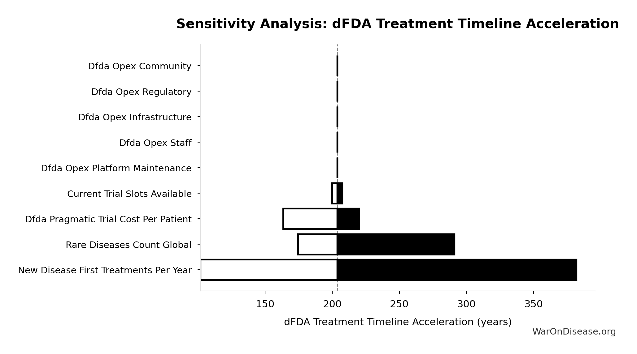
Sensitivity Analysis
Sensitivity Indices for dFDA Treatment Timeline Acceleration
Regression-based sensitivity showing which inputs explain the most variance in the output.
| Input Parameter | Sensitivity Coefficient | Interpretation |
|---|---|---|
| Status Quo Average Years to First Treatment (years) | 1.0664 | Strong driver |
| Trial Capacity Multiplier (x) | -0.0777 | Minimal effect |
Interpretation: Standardized coefficients show the change in output (in SD units) per 1 SD change in input. Values near ±1 indicate strong influence; values exceeding ±1 may occur with correlated inputs.
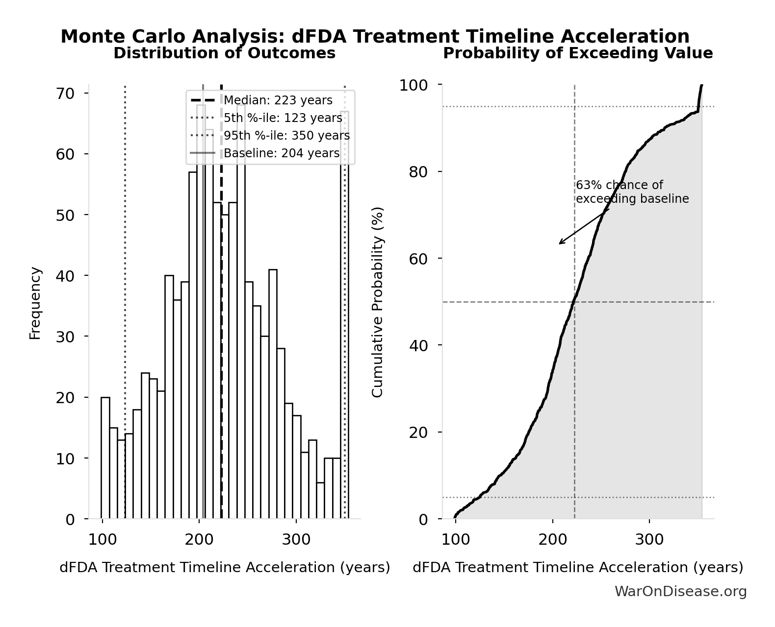
Monte Carlo Distribution
Simulation Results Summary: dFDA Treatment Timeline Acceleration
| Statistic | Value |
|---|---|
| Baseline (deterministic) | 204 |
| Mean (expected value) | 225 |
| Median (50th percentile) | 223 |
| Standard Deviation | 62.3 |
| 90% Range (5th-95th percentile) | [123, 350] |
The histogram shows the distribution of dFDA Treatment Timeline Acceleration across 10,000 Monte Carlo simulations. The CDF (right) shows the probability of the outcome exceeding any given value, which is useful for risk assessment.
Exceedance Probability
This exceedance probability chart shows the likelihood that dFDA Treatment Timeline Acceleration will exceed any given threshold. Higher curves indicate more favorable outcomes with greater certainty.
dFDA Annual Trial Subsidies: $21.8B
Note📊 Details
Annual clinical trial patient subsidies from dFDA funding (total funding minus operational costs)
Inputs:
- dFDA Annual Trial Funding: $21.8B
- Total Annual Decentralized Framework for Drug Assessment Operational Costs 🔢: $40M
\[ \begin{gathered} Subsidies_{dFDA,ann} \\ = Funding_{dFDA,ann} - OPEX_{dFDA} \\ = \$21.8B - \$40M \\ = \$21.8B \end{gathered} \] where: \[ \begin{gathered} OPEX_{dFDA} \\ = Cost_{platform} + Cost_{staff} + Cost_{infra} \\ + Cost_{regulatory} + Cost_{community} \\ = \$15M + \$10M + \$8M + \$5M + \$2M \\ = \$40M \end{gathered} \] ✓ High confidence
Sensitivity Analysis
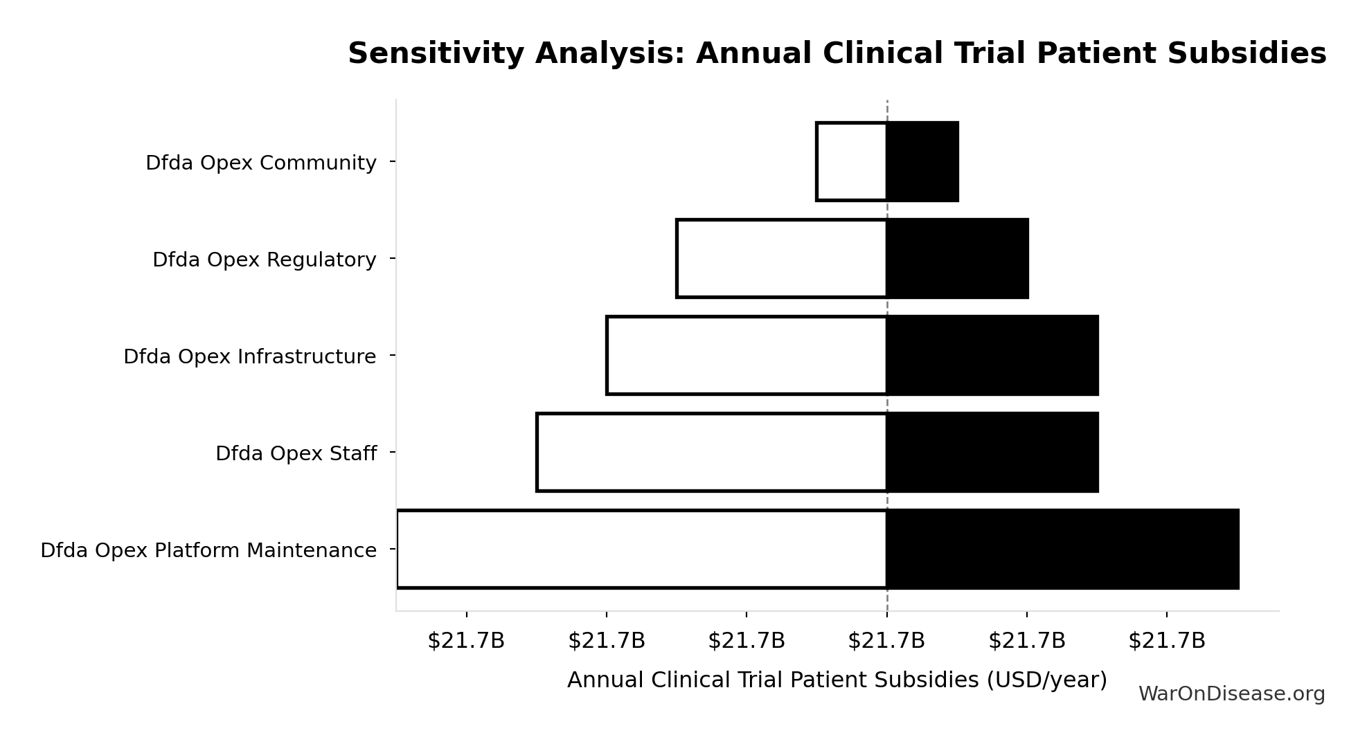
Sensitivity Indices for dFDA Annual Trial Subsidies
Regression-based sensitivity showing which inputs explain the most variance in the output.
| Input Parameter | Sensitivity Coefficient | Interpretation |
|---|---|---|
| Total Annual Decentralized Framework for Drug Assessment Operational Costs (USD/year) | -1.0000 | Strong driver |
Interpretation: Standardized coefficients show the change in output (in SD units) per 1 SD change in input. Values near ±1 indicate strong influence; values exceeding ±1 may occur with correlated inputs.
Monte Carlo Distribution
Simulation Results Summary: dFDA Annual Trial Subsidies
| Statistic | Value |
|---|---|
| Baseline (deterministic) | $21.8B |
| Mean (expected value) | $21.8B |
| Median (50th percentile) | $21.8B |
| Standard Deviation | $8.21M |
| 90% Range (5th-95th percentile) | [$21.7B, $21.8B] |
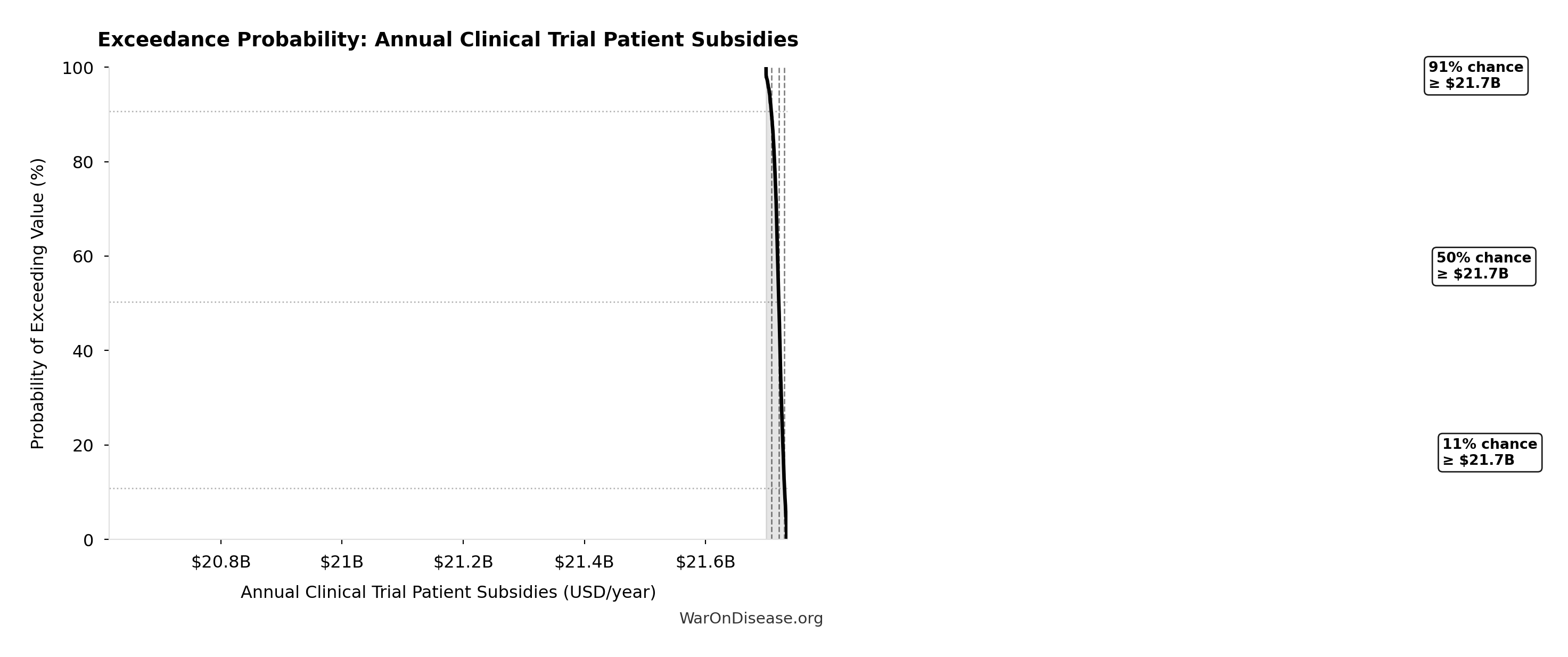
The histogram shows the distribution of dFDA Annual Trial Subsidies across 10,000 Monte Carlo simulations. The CDF (right) shows the probability of the outcome exceeding any given value, which is useful for risk assessment.
Exceedance Probability
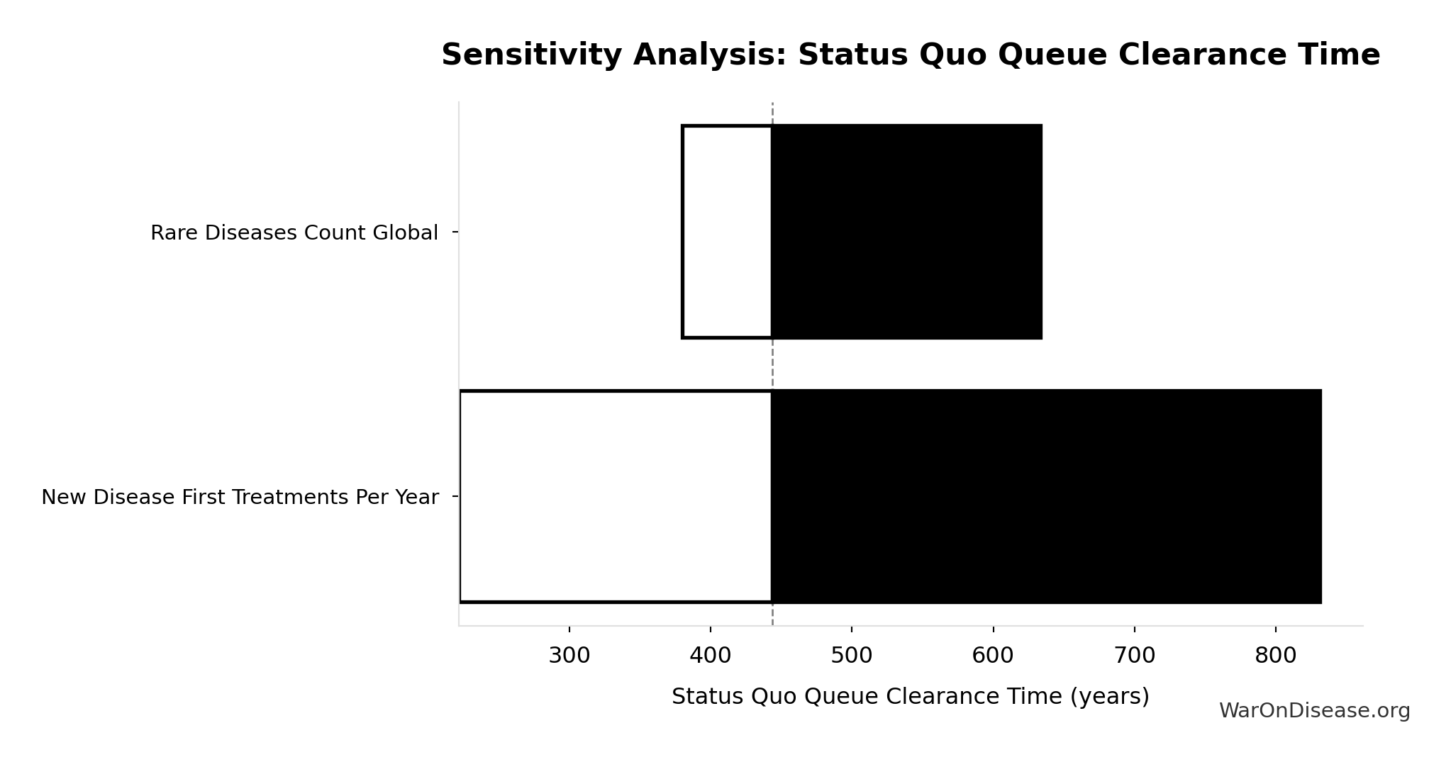
This exceedance probability chart shows the likelihood that dFDA Annual Trial Subsidies will exceed any given threshold. Higher curves indicate more favorable outcomes with greater certainty.
Diseases Without Effective Treatment: 6.65 thousand diseases
Note📊 Details
Number of diseases without effective treatment. 95% of 7,000 rare diseases lack FDA-approved treatment (per Orphanet 2024). This represents the therapeutic search space that remains unexplored.
Inputs:
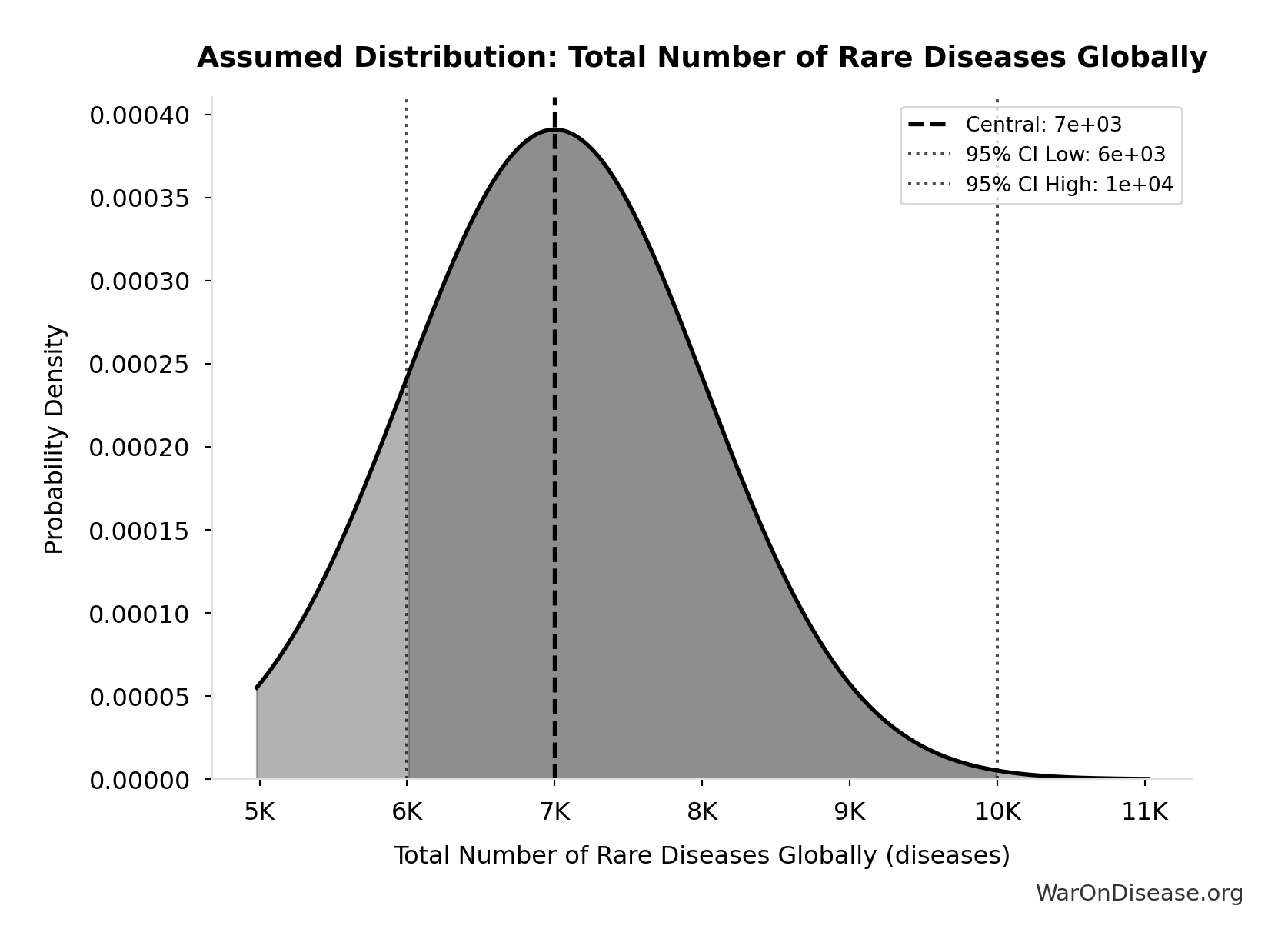
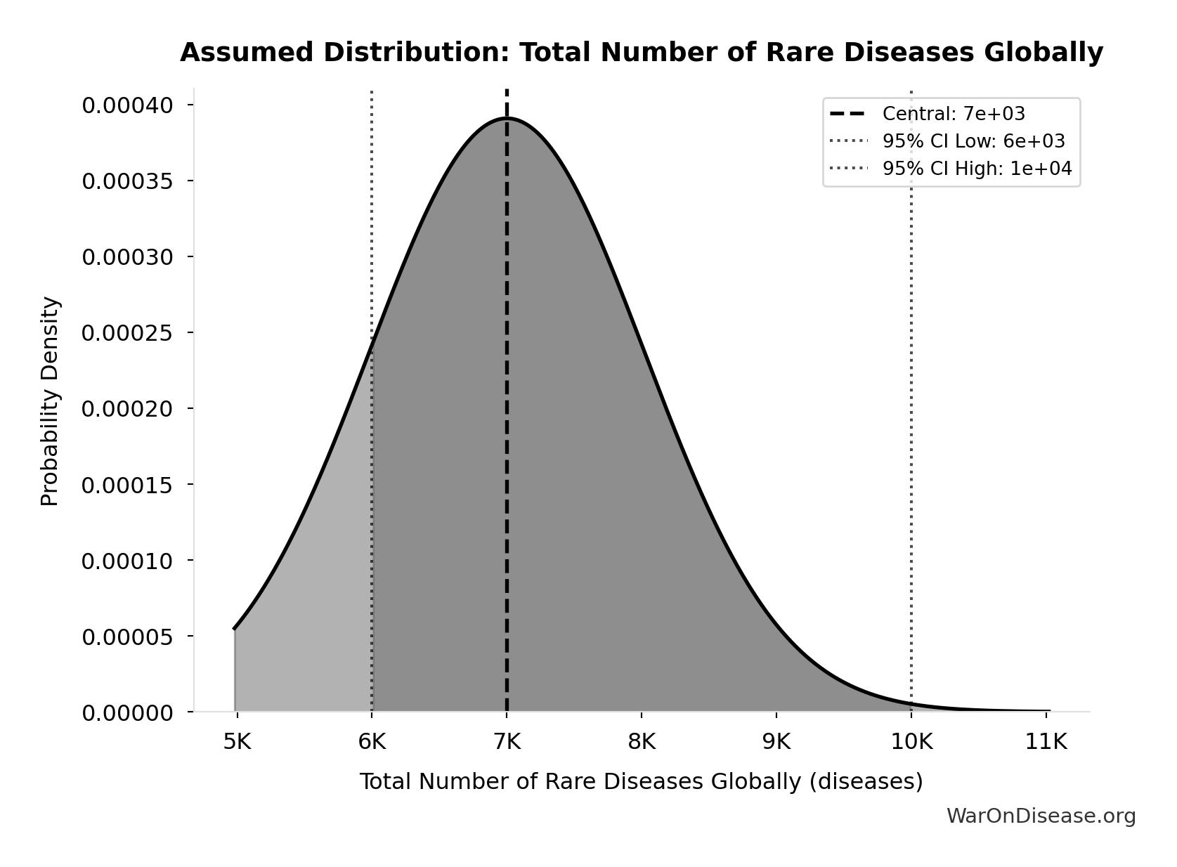
- Total Number of Rare Diseases Globally 📊: 7 thousand diseases (95% CI: 6 thousand diseases - 10 thousand diseases)
\[ \begin{gathered} N_{untreated} \\ = N_{rare} \times 0.95 \\ = 7{,}000 \times 0.95 \\ = 6{,}650 \end{gathered} \]
Methodology:139
~ Medium confidence
Sensitivity Analysis
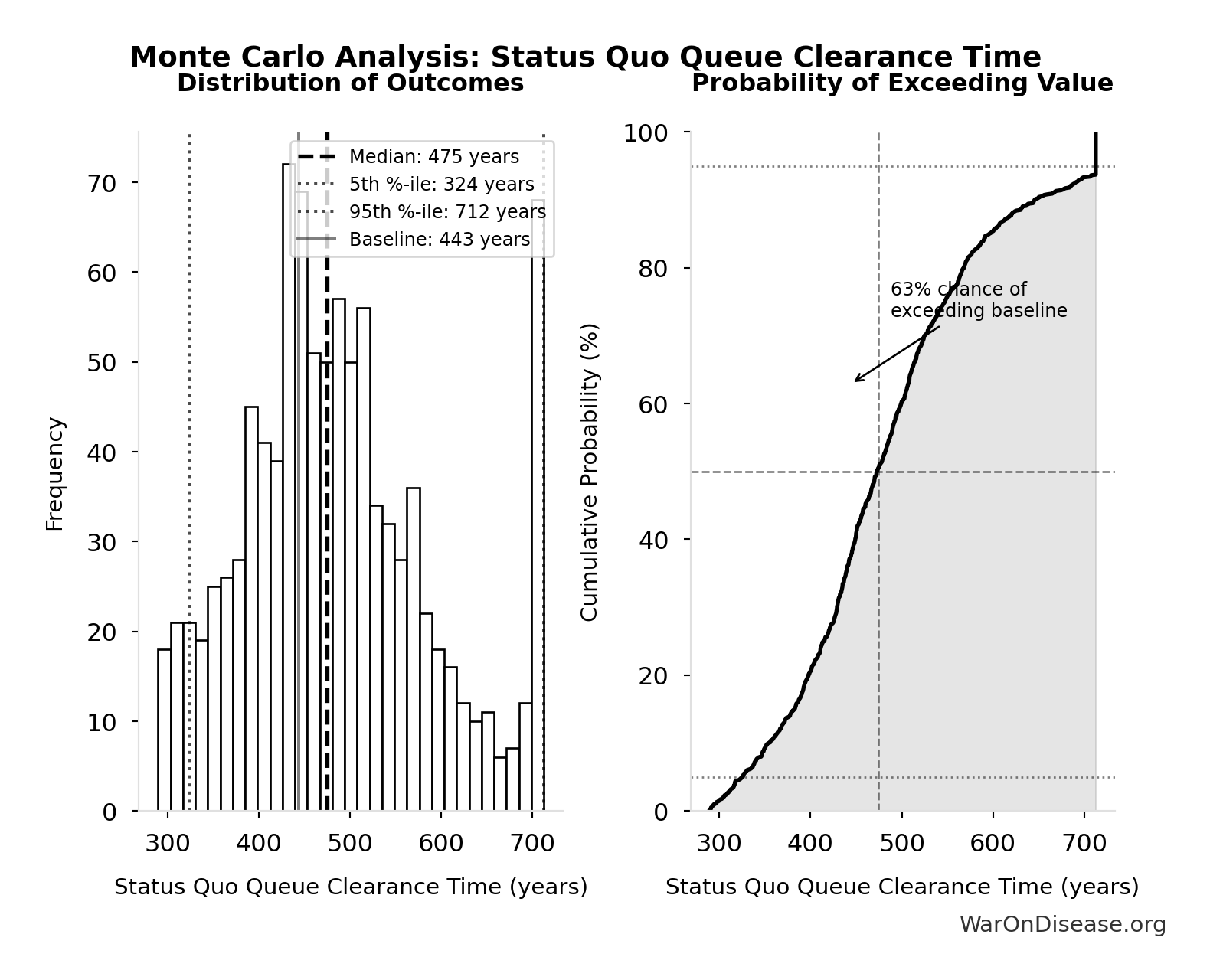
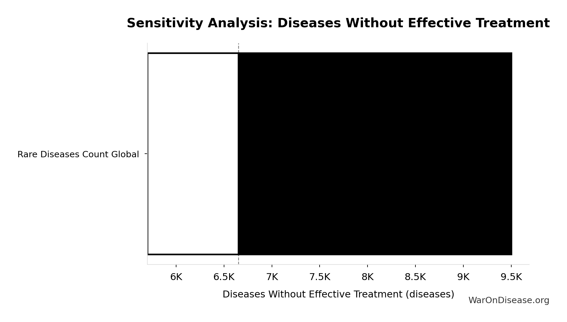
Sensitivity Indices for Diseases Without Effective Treatment
Regression-based sensitivity showing which inputs explain the most variance in the output.
| Input Parameter | Sensitivity Coefficient | Interpretation |
|---|---|---|
| Total Number of Rare Diseases Globally (diseases) | 1.0000 | Strong driver |
Interpretation: Standardized coefficients show the change in output (in SD units) per 1 SD change in input. Values near ±1 indicate strong influence; values exceeding ±1 may occur with correlated inputs.
Monte Carlo Distribution
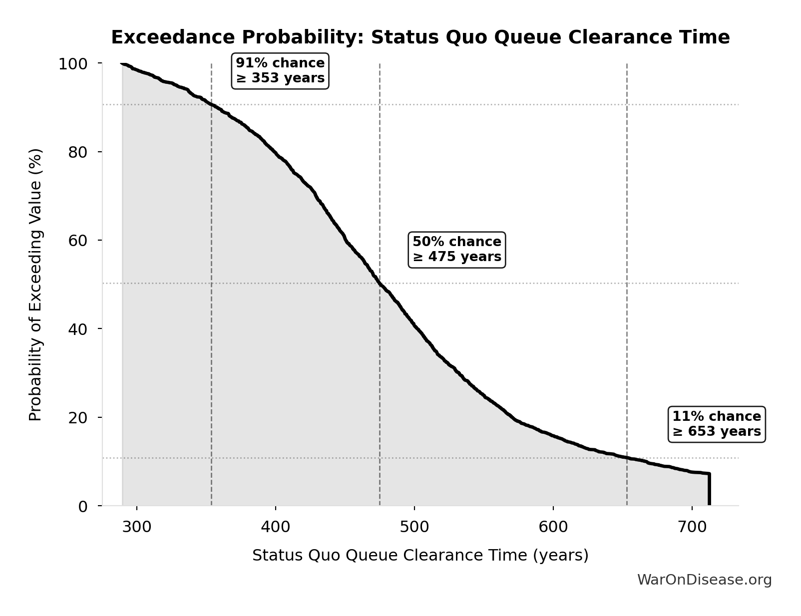
Simulation Results Summary: Diseases Without Effective Treatment
| Statistic | Value |
|---|---|
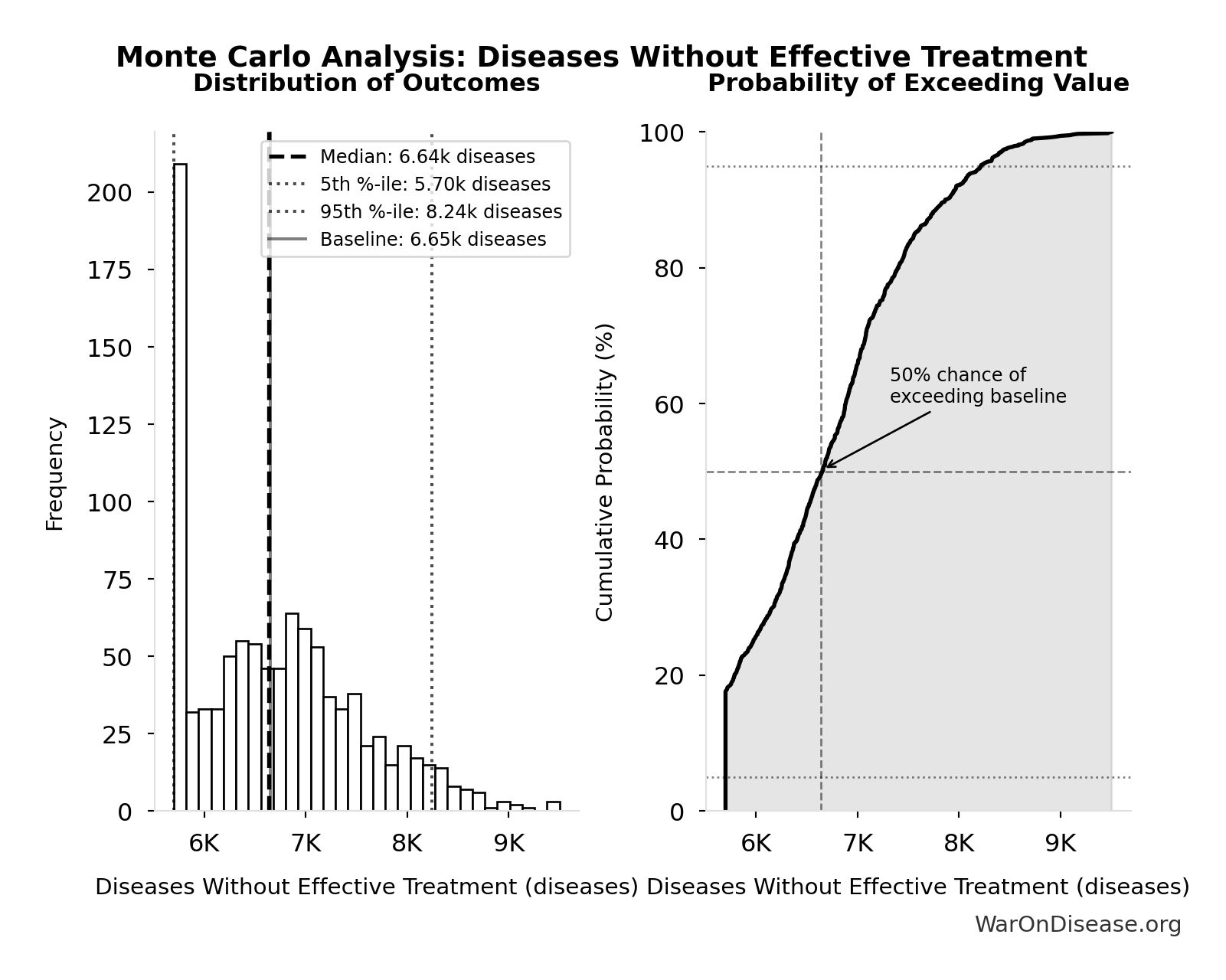
| Baseline (deterministic) | 6.65 thousand |
| Mean (expected value) | 6.73 thousand |
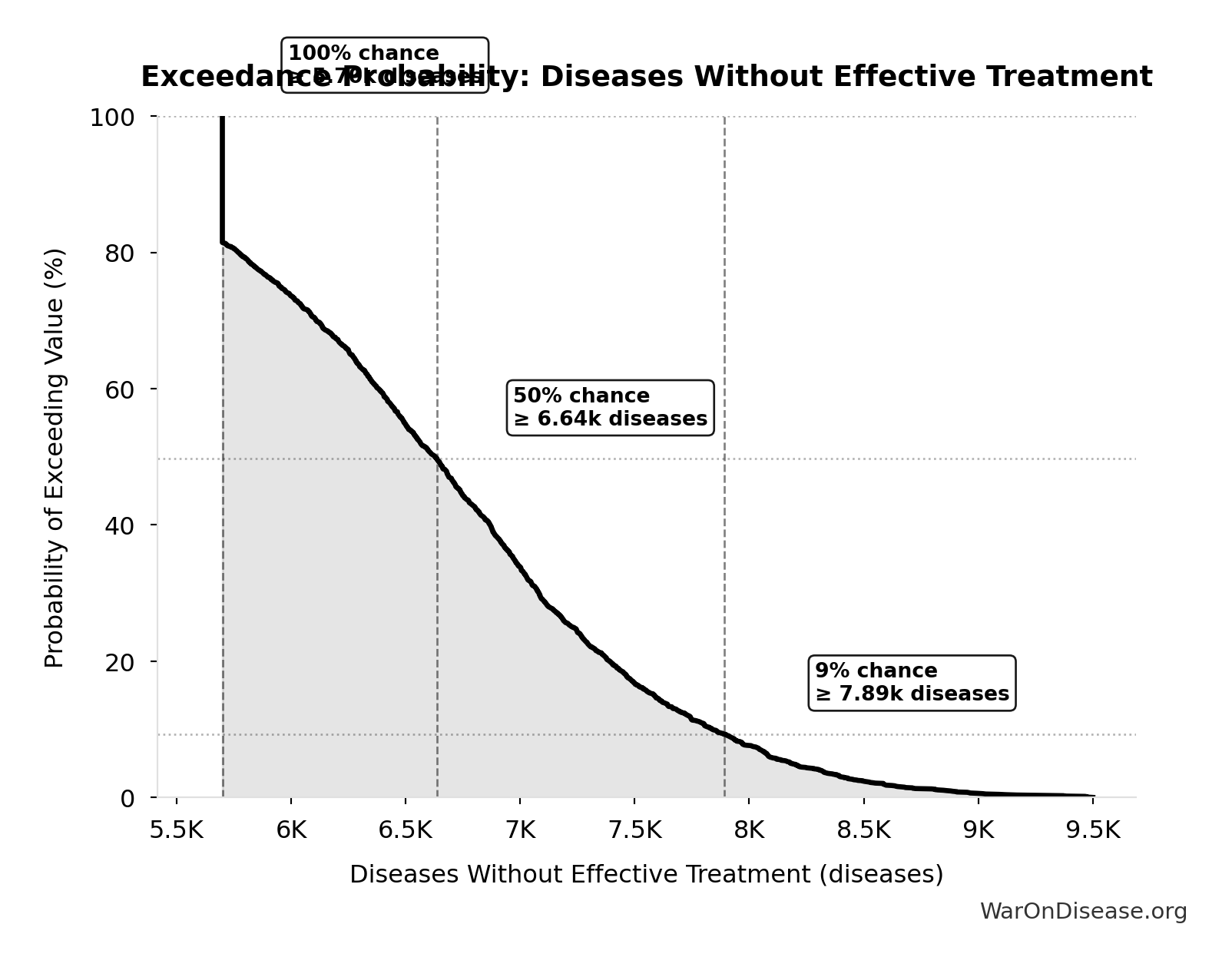
| Median (50th percentile) | 6.64 thousand |
| Standard Deviation | 835 |
| 90% Range (5th-95th percentile) | [5.7 thousand, 8.24 thousand] |
The histogram shows the distribution of Diseases Without Effective Treatment across 10,000 Monte Carlo simulations. The CDF (right) shows the probability of the outcome exceeding any given value, which is useful for risk assessment.
Exceedance Probability
This exceedance probability chart shows the likelihood that Diseases Without Effective Treatment will exceed any given threshold. Higher curves indicate more favorable outcomes with greater certainty.
Global Political Reform Investment: $128B
Note📊 Details
Estimated global advocacy investment for policy reform. Calculated as US costs × global ratio (based on discretionary spending). Upper bound representing full democratic engagement at scale.
Inputs:
- US Political Reform Investment (Total) 🔢: $25.5B
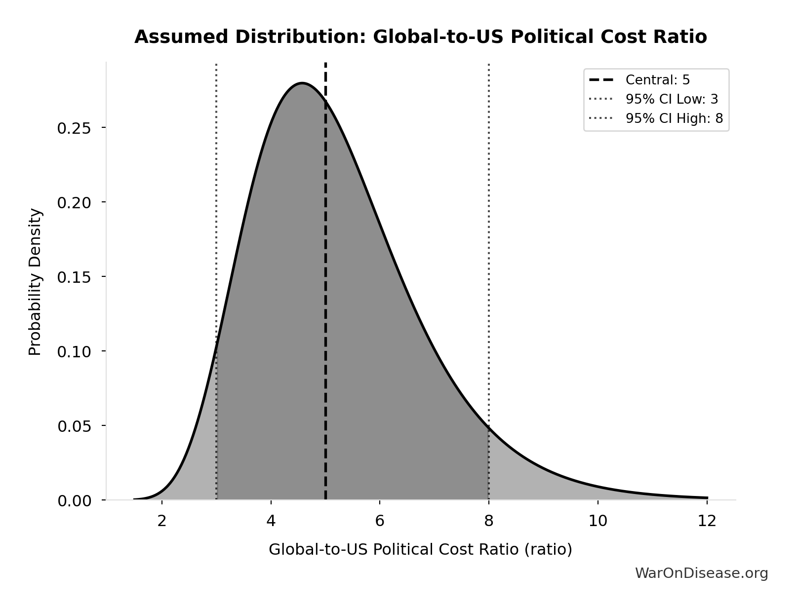
- Global-to-US Political Cost Ratio: 5:1 (95% CI: 3:1 - 8:1)
\[ \begin{gathered} Cost_{global,reform} \\ = Cost_{US,total} \times \rho_{global/US} \\ = \$25.5B \times 5 \\ = \$128B \end{gathered} \] where: \[ \begin{gathered} Cost_{US,total} \\ = (Cost_{campaign} \\ + Cost_{lobby} \times 2) \times \mu_{effort} + Cost_{career} \end{gathered} \] where: \[ \begin{gathered} Cost_{US,congress} \\ = N_{congress} \times V_{post-office} \\ = 535 \times \$10M \\ = \$5.35B \end{gathered} \] ? Low confidence
Sensitivity Analysis
Sensitivity Indices for Global Political Reform Investment
Regression-based sensitivity showing which inputs explain the most variance in the output.
| Input Parameter | Sensitivity Coefficient | Interpretation |
|---|---|---|
| US Political Reform Investment (Total) (USD) | 4.7165 | Strong driver |
| Global-to-US Political Cost Ratio (ratio) | -3.7249 | Strong driver |
Interpretation: Standardized coefficients show the change in output (in SD units) per 1 SD change in input. Values near ±1 indicate strong influence; values exceeding ±1 may occur with correlated inputs.
Monte Carlo Distribution
Simulation Results Summary: Global Political Reform Investment
| Statistic | Value |
|---|---|
| Baseline (deterministic) | $128B |
| Mean (expected value) | $133B |
| Median (50th percentile) | $119B |
| Standard Deviation | $62.7B |
| 90% Range (5th-95th percentile) | [$55.2B, $266B] |
The histogram shows the distribution of Global Political Reform Investment across 10,000 Monte Carlo simulations. The CDF (right) shows the probability of the outcome exceeding any given value, which is useful for risk assessment.
Exceedance Probability
This exceedance probability chart shows the likelihood that Global Political Reform Investment will exceed any given threshold. Higher curves indicate more favorable outcomes with greater certainty.
Global Opportunity Cost Total: $101T
Note📊 Details
Total global opportunity cost from governance failures: health innovation delays ($34T), underfunded science ($4T), lead poisoning ($6T), migration restrictions ($57T). Sum: $101T annually in unrealized potential.
Inputs:
- Global Health Opportunity Cost 📊: $34T (95% CI: $20T - $80T)
- Global Science Opportunity Cost 📊: $4T (95% CI: $2T - $10T)
- Global Lead Poisoning Cost 📊: $6T (95% CI: $4T - $8T)
- Global Migration Opportunity Cost 📊: $57T (95% CI: $57T - $170T)
\[ \begin{gathered} O_{total} \\ = O_{health} + O_{science} + O_{lead} + O_{migration} \\ = \$34T + \$4T + \$6T + \$57T \\ = \$101T \end{gathered} \]
Methodology:47
? Low confidence
Sensitivity Analysis
Sensitivity Indices for Global Opportunity Cost Total
Regression-based sensitivity showing which inputs explain the most variance in the output.
| Input Parameter | Sensitivity Coefficient | Interpretation |
|---|---|---|
| Global Migration Opportunity Cost (USD) | 0.5736 | Strong driver |
| Global Health Opportunity Cost (USD) | 0.3734 | Moderate driver |
| Global Science Opportunity Cost (USD) | 0.0500 | Minimal effect |
| Global Lead Poisoning Cost (USD) | 0.0264 | Minimal effect |
Interpretation: Standardized coefficients show the change in output (in SD units) per 1 SD change in input. Values near ±1 indicate strong influence; values exceeding ±1 may occur with correlated inputs.
Monte Carlo Distribution
Simulation Results Summary: Global Opportunity Cost Total
| Statistic | Value |
|---|---|
| Baseline (deterministic) | $101T |
| Mean (expected value) | $112T |
| Median (50th percentile) | $97.5T |
| Standard Deviation | $36.5T |
| 90% Range (5th-95th percentile) | [$83.3T, $191T] |
The histogram shows the distribution of Global Opportunity Cost Total across 10,000 Monte Carlo simulations. The CDF (right) shows the probability of the outcome exceeding any given value, which is useful for risk assessment.
Exceedance Probability
This exceedance probability chart shows the likelihood that Global Opportunity Cost Total will exceed any given threshold. Higher curves indicate more favorable outcomes with greater certainty.
Percentage Military Spending Cut After WW2: 87.6%
Note📊 Details
Percentage US military spending cut after WW2 (1945-1947, inflation-adjusted: $1,420B to $176B in constant 2024 dollars)
Inputs:
- US Military Spending in 1947 (Constant 2024 Dollars) 📊: $176B
- US Military Spending at WW2 Peak (Constant 2024 Dollars) 📊: $1.42T
\[ \begin{gathered} Cut_{WW2} \\ = 1 - \frac{Spending_{US,1947}}{Spending_{US,1945}} \\ = 1 - \frac{\$176B}{\$1.42T} \\ = 87.6\% \end{gathered} \]
✓ High confidence
Status Quo Average Years to First Treatment: 222 years
Note📊 Details
Average years until first treatment discovered for a typical disease under current system. At current discovery rates, the average disease waits half the total exploration time (~443/2 = ~222 years).
Inputs:
- Status Quo Therapeutic Space Exploration Time 🔢: 443 years
\[ \begin{gathered} T_{first,SQ} \\ = T_{queue,SQ} \times 0.5 \\ = 443 \times 0.5 \\ = 222 \end{gathered} \] where: \[ \begin{gathered} T_{queue,SQ} \\ = \frac{N_{untreated}}{Treatments_{new,ann}} \\ = \frac{6{,}650}{15} \\ = 443 \end{gathered} \] where: \[ \begin{gathered} N_{untreated} \\ = N_{rare} \times 0.95 \\ = 7{,}000 \times 0.95 \\ = 6{,}650 \end{gathered} \] Methodology:140
? Low confidence
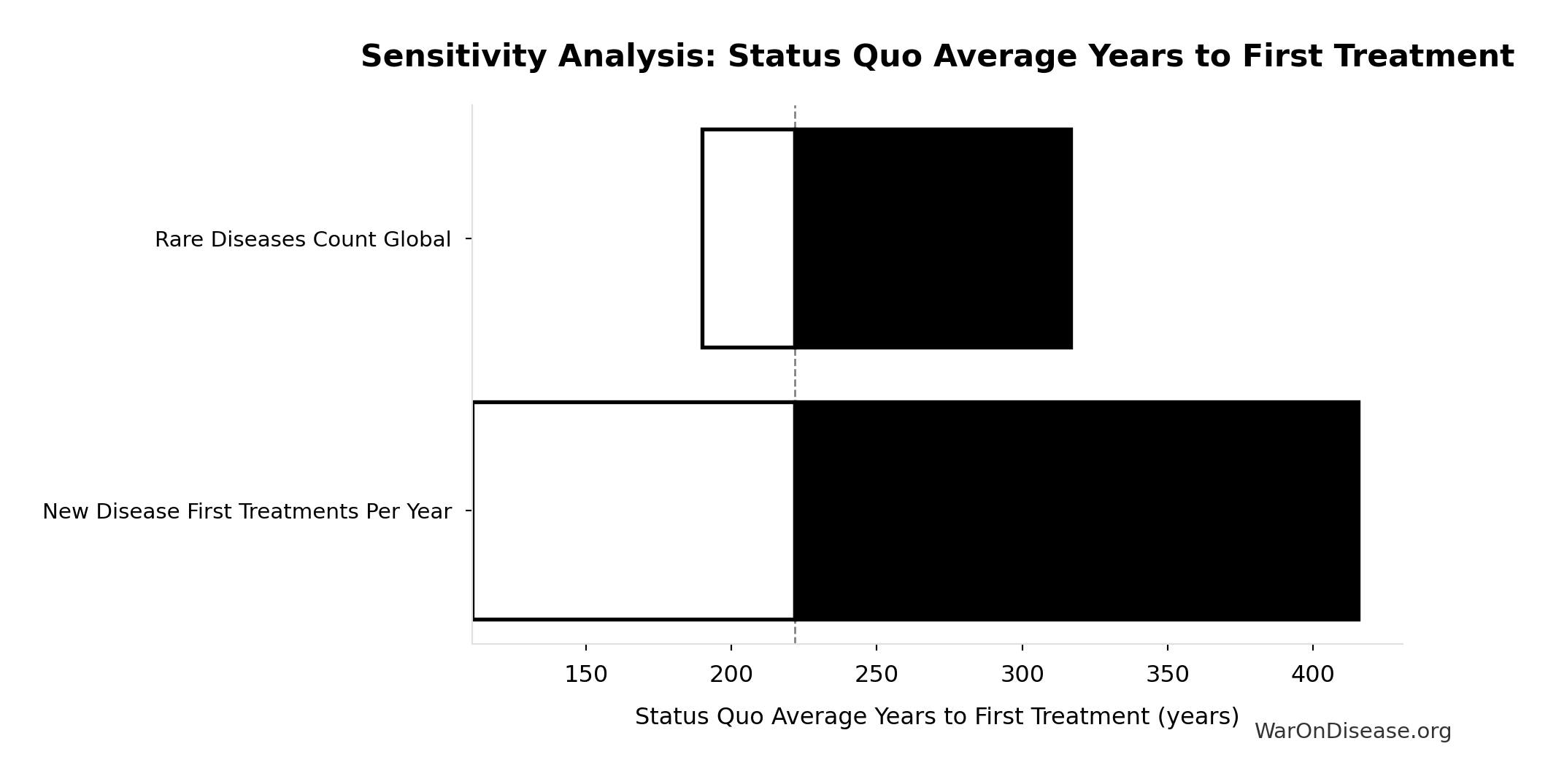
Sensitivity Analysis
Sensitivity Indices for Status Quo Average Years to First Treatment
Regression-based sensitivity showing which inputs explain the most variance in the output.
| Input Parameter | Sensitivity Coefficient | Interpretation |
|---|---|---|
| Status Quo Therapeutic Space Exploration Time (years) | 1.0000 | Strong driver |
Interpretation: Standardized coefficients show the change in output (in SD units) per 1 SD change in input. Values near ±1 indicate strong influence; values exceeding ±1 may occur with correlated inputs.
Monte Carlo Distribution
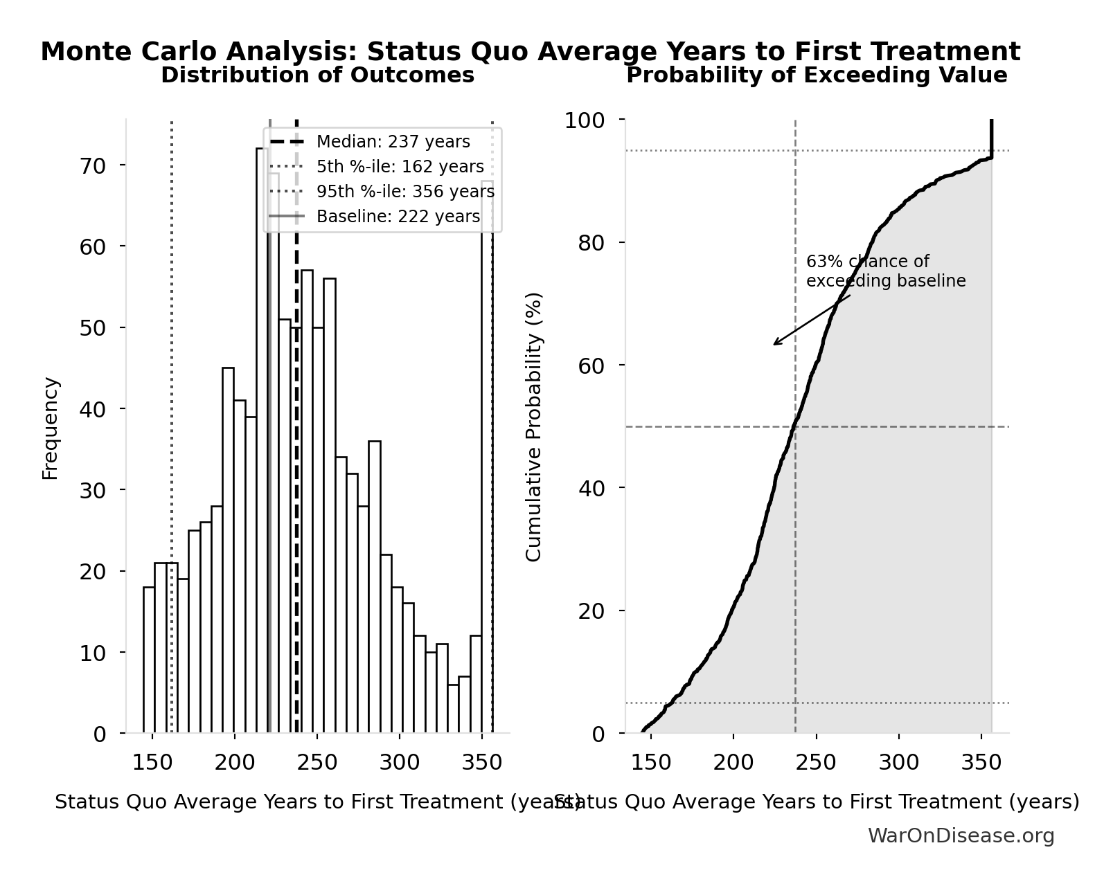
Simulation Results Summary: Status Quo Average Years to First Treatment
| Statistic | Value |
|---|---|
| Baseline (deterministic) | 222 |
| Mean (expected value) | 242 |
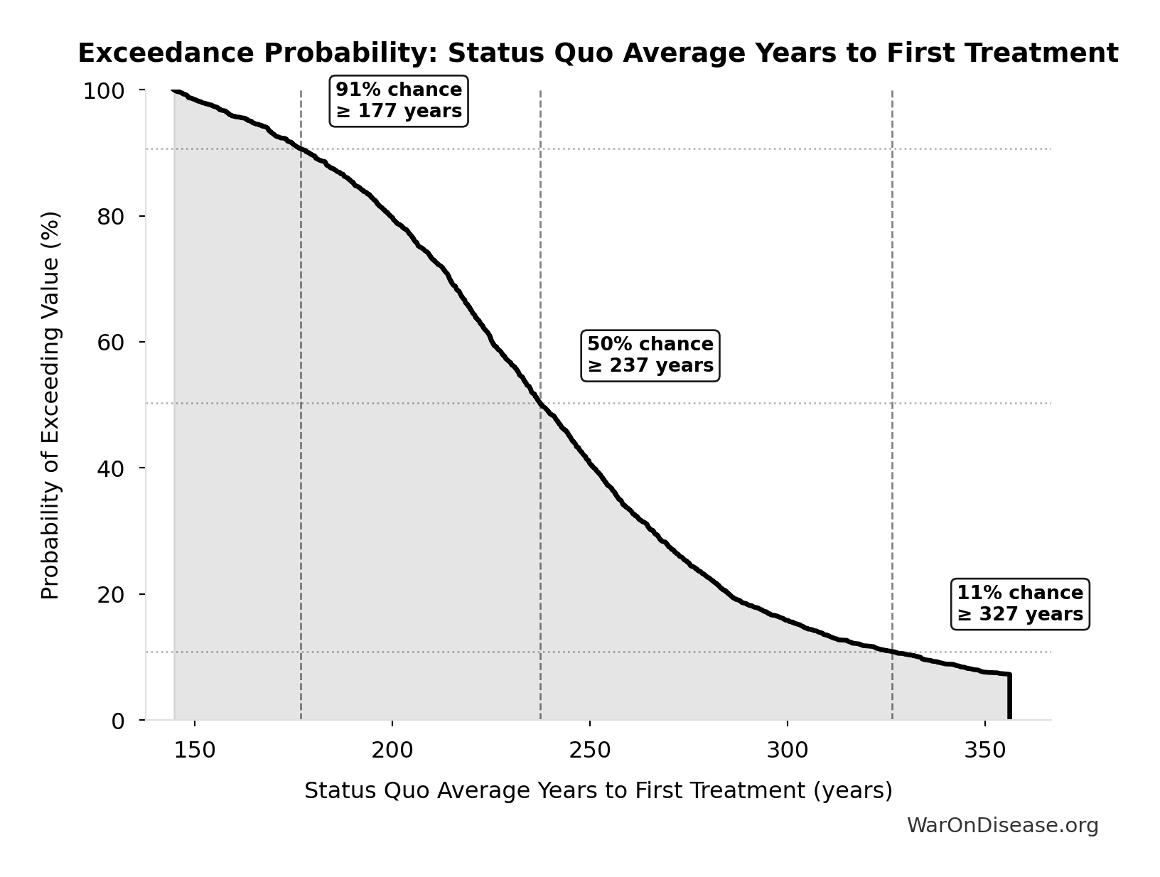
| Median (50th percentile) | 237 |
| Standard Deviation | 53.2 |
| 90% Range (5th-95th percentile) | [162, 356] |
The histogram shows the distribution of Status Quo Average Years to First Treatment across 10,000 Monte Carlo simulations. The CDF (right) shows the probability of the outcome exceeding any given value, which is useful for risk assessment.
Exceedance Probability
This exceedance probability chart shows the likelihood that Status Quo Average Years to First Treatment will exceed any given threshold. Higher curves indicate more favorable outcomes with greater certainty.
Status Quo Therapeutic Space Exploration Time: 443 years
Note📊 Details
Years to explore the entire therapeutic search space under current system. At current discovery rate of ~15 diseases/year getting first treatments, finding treatments for all ~6,650 untreated diseases would take ~443 years.
Inputs:
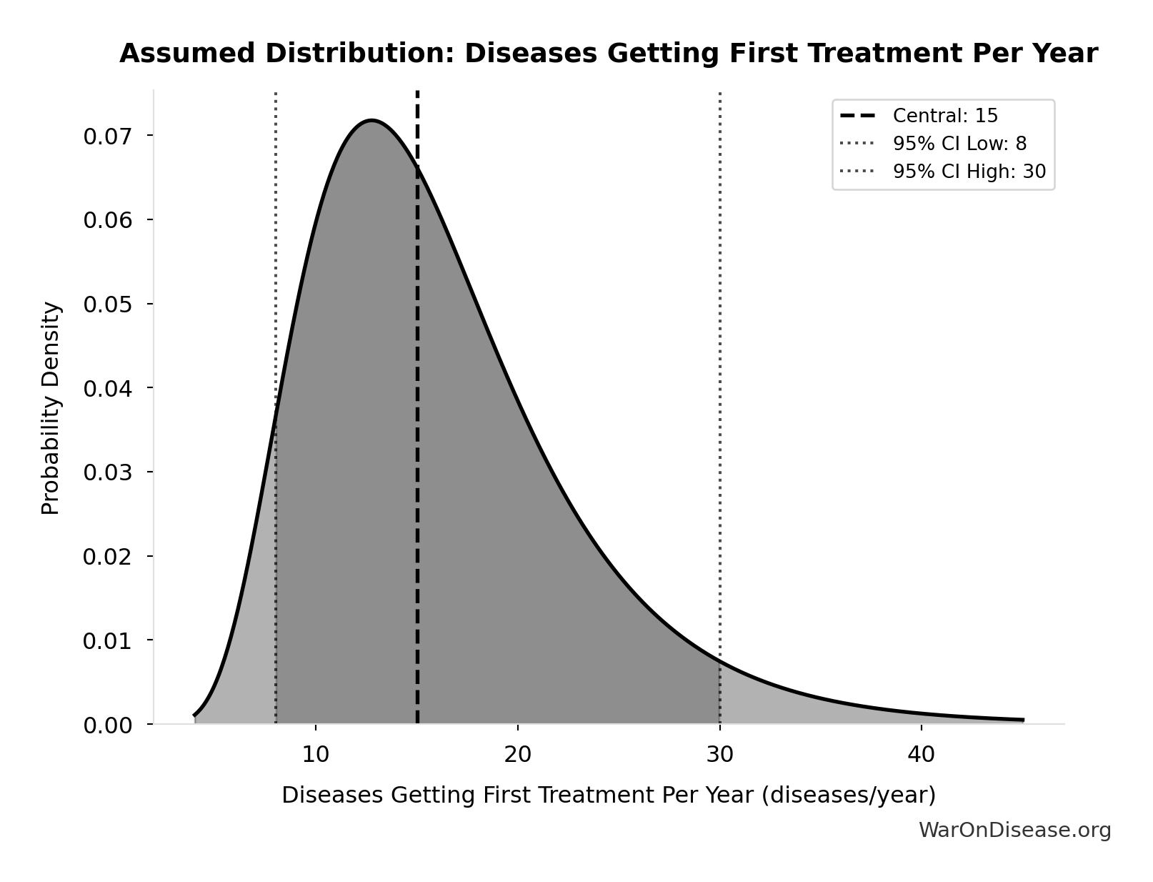
- Diseases Without Effective Treatment 🔢: 6.65 thousand diseases
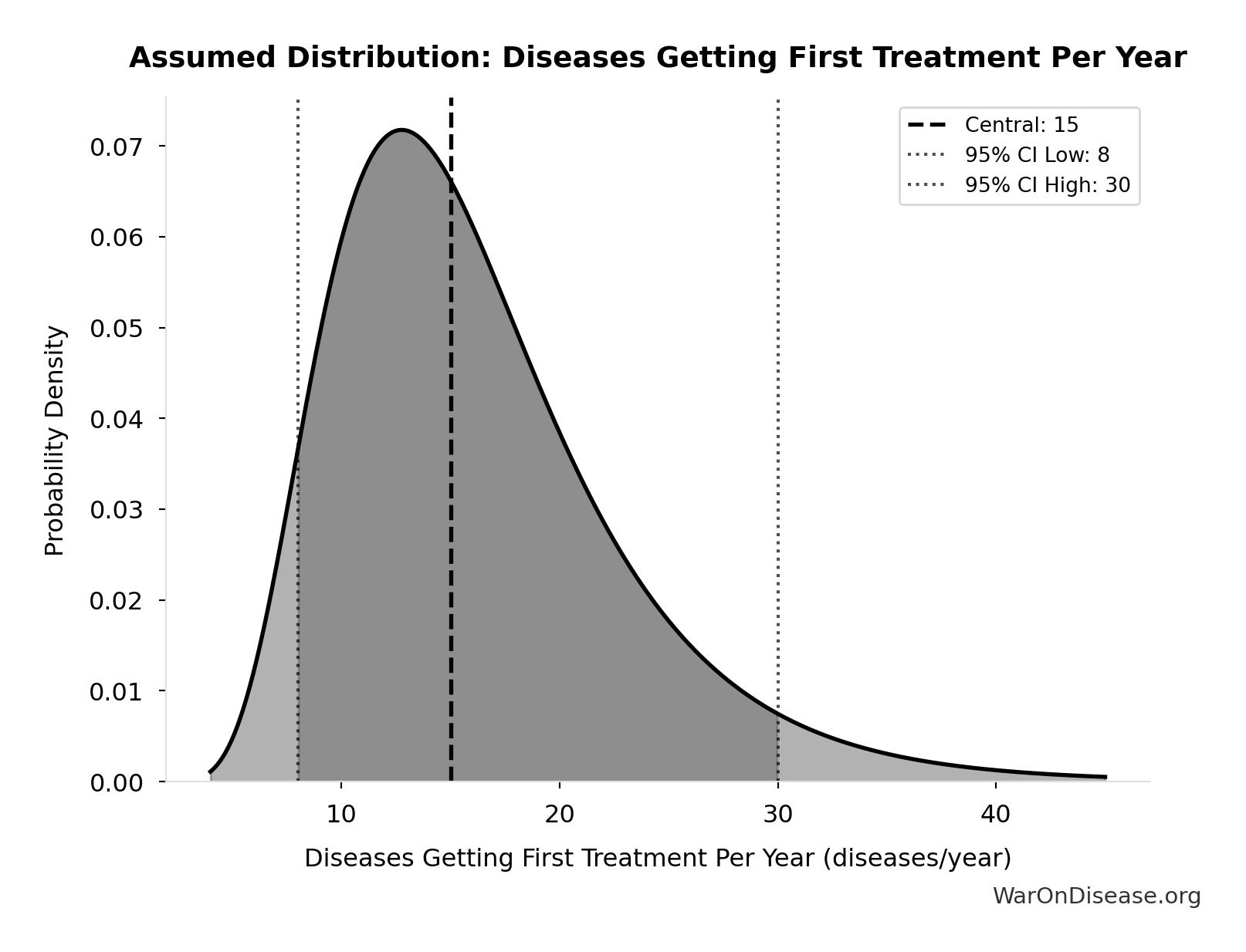
- Diseases Getting First Treatment Per Year 📊: 15 diseases/year (95% CI: 8 diseases/year - 30 diseases/year)
\[ \begin{gathered} T_{queue,SQ} \\ = \frac{N_{untreated}}{Treatments_{new,ann}} \\ = \frac{6{,}650}{15} \\ = 443 \end{gathered} \] where: \[ \begin{gathered} N_{untreated} \\ = N_{rare} \times 0.95 \\ = 7{,}000 \times 0.95 \\ = 6{,}650 \end{gathered} \] Methodology:140
? Low confidence
Sensitivity Analysis
Sensitivity Indices for Status Quo Therapeutic Space Exploration Time
Regression-based sensitivity showing which inputs explain the most variance in the output.
| Input Parameter | Sensitivity Coefficient | Interpretation |
|---|---|---|
| Diseases Without Effective Treatment (diseases) | -0.7011 | Strong driver |
| Diseases Getting First Treatment Per Year (diseases/year) | -0.2360 | Weak driver |
Interpretation: Standardized coefficients show the change in output (in SD units) per 1 SD change in input. Values near ±1 indicate strong influence; values exceeding ±1 may occur with correlated inputs.
Monte Carlo Distribution
Simulation Results Summary: Status Quo Therapeutic Space Exploration Time
| Statistic | Value |
|---|---|
| Baseline (deterministic) | 443 |
| Mean (expected value) | 485 |
| Median (50th percentile) | 475 |
| Standard Deviation | 106 |
| 90% Range (5th-95th percentile) | [324, 712] |
The histogram shows the distribution of Status Quo Therapeutic Space Exploration Time across 10,000 Monte Carlo simulations. The CDF (right) shows the probability of the outcome exceeding any given value, which is useful for risk assessment.
Exceedance Probability
This exceedance probability chart shows the likelihood that Status Quo Therapeutic Space Exploration Time will exceed any given threshold. Higher curves indicate more favorable outcomes with greater certainty.
Annual Funding from 1% of Global Military Spending Redirected to DIH: $27.2B
Note📊 Details
Annual funding from 1% of global military spending redirected to DIH
Inputs:
- Global Military Spending in 2024 📊: $2.72T
- 1% Reduction in Military Spending/War Costs from Treaty: 1%
\[ \begin{gathered} Funding_{treaty} \\ = Spending_{mil} \times Reduce_{treaty} \\ = \$2.72T \times 1\% \\ = \$27.2B \end{gathered} \]
✓ High confidence
Total 1% Treaty Campaign Cost: $1B
Note📊 Details
Total treaty campaign cost (100% VICTORY Incentive Alignment Bonds)
Inputs:
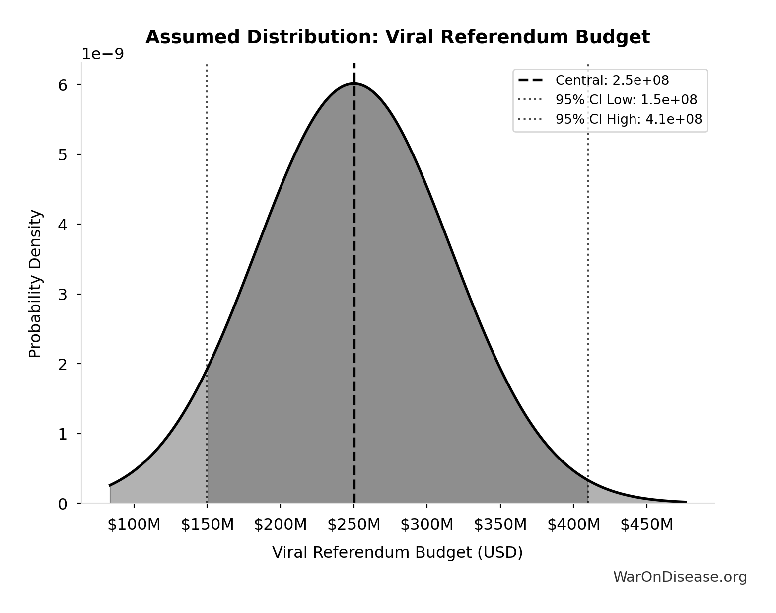
- Viral Referendum Budget: $250M (95% CI: $150M - $410M)
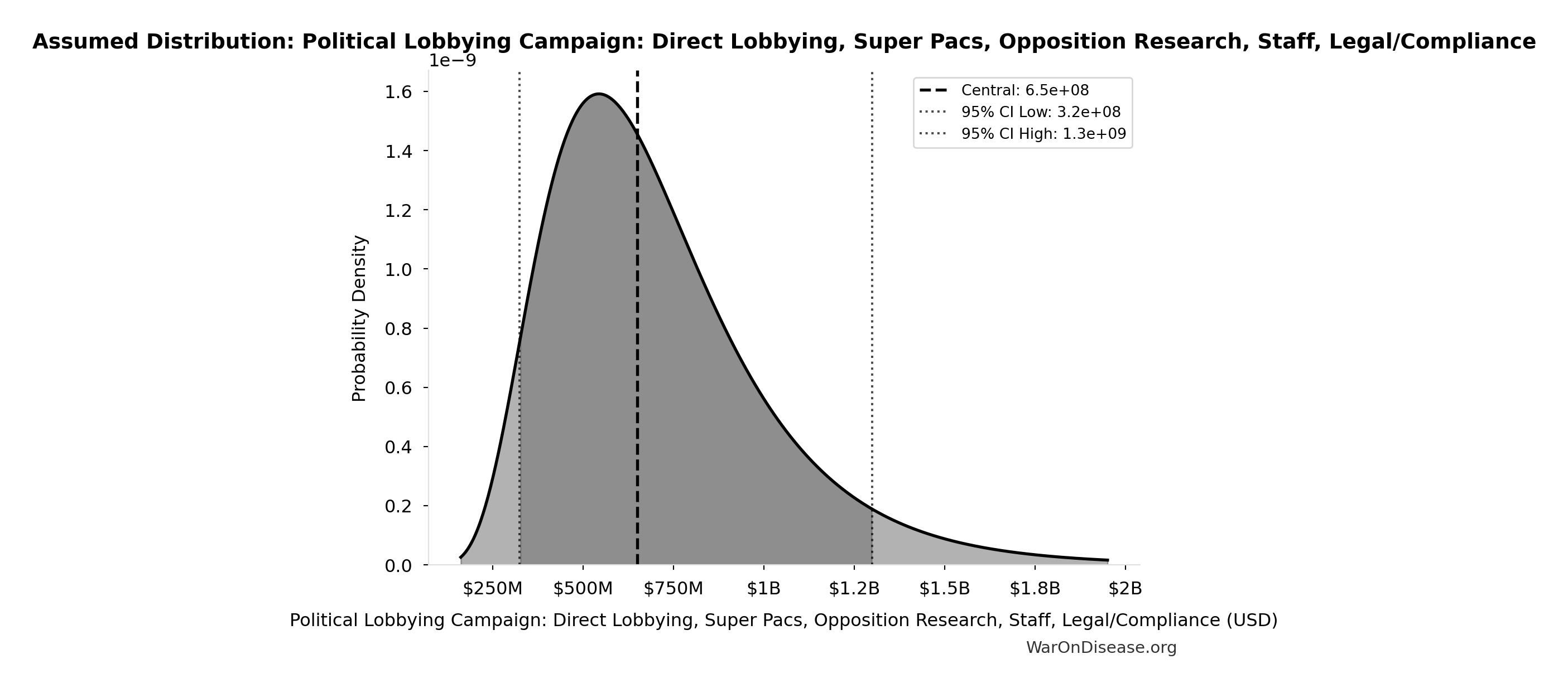
- Political Lobbying Campaign: Direct Lobbying, Super Pacs, Opposition Research, Staff, Legal/Compliance: $650M (95% CI: $325M - $1.3B)
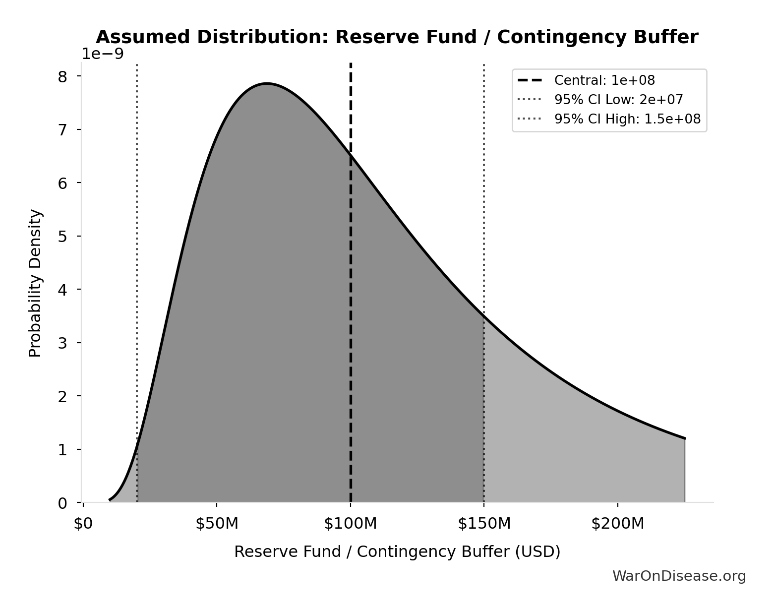
- Reserve Fund / Contingency Buffer: $100M (95% CI: $20M - $150M)
\[ \begin{gathered} Cost_{campaign} \\ = Budget_{viral,base} + Budget_{lobby,treaty} \\ + Budget_{reserve} \\ = \$250M + \$650M + \$100M \\ = \$1B \end{gathered} \]
✓ High confidence
Sensitivity Analysis
Sensitivity Indices for Total 1% Treaty Campaign Cost
Regression-based sensitivity showing which inputs explain the most variance in the output.
| Input Parameter | Sensitivity Coefficient | Interpretation |
|---|---|---|
| Political Lobbying Campaign: Direct Lobbying, Super Pacs, Opposition Research, Staff, Legal/Compliance (USD) | 0.9016 | Strong driver |
| Reserve Fund / Contingency Buffer (USD) | 0.1026 | Weak driver |
Interpretation: Standardized coefficients show the change in output (in SD units) per 1 SD change in input. Values near ±1 indicate strong influence; values exceeding ±1 may occur with correlated inputs.
Monte Carlo Distribution
Simulation Results Summary: Total 1% Treaty Campaign Cost
| Statistic | Value |
|---|---|
| Baseline (deterministic) | $1B |
| Mean (expected value) | $996M |
| Median (50th percentile) | $949M |
| Standard Deviation | $276M |
| 90% Range (5th-95th percentile) | [$632M, $1.51B] |
The histogram shows the distribution of Total 1% Treaty Campaign Cost across 10,000 Monte Carlo simulations. The CDF (right) shows the probability of the outcome exceeding any given value, which is useful for risk assessment.
Exceedance Probability
This exceedance probability chart shows the likelihood that Total 1% Treaty Campaign Cost will exceed any given threshold. Higher curves indicate more favorable outcomes with greater certainty.
Cost per DALY Averted (Elimination of Efficacy Lag Plus Earlier Treatment Discovery from Increased Trial Throughput): $0.00177
Note📊 Details
Cost per DALY averted from elimination of efficacy lag plus earlier treatment discovery from increased trial throughput. Only counts campaign cost; ignores economic benefits from funding and R&D savings.
Inputs:
- Total 1% Treaty Campaign Cost 🔢: $1B
- Total DALYs from Elimination of Efficacy Lag Plus Earlier Treatment Discovery from Higher Trial Throughput 🔢: 565 billion DALYs
\[ \begin{gathered} Cost_{treaty,DALY} \\ = \frac{Cost_{campaign}}{DALYs_{max}} \\ = \frac{\$1B}{565B} \\ = \$0.00177 \end{gathered} \] where: \[ \begin{gathered} Cost_{campaign} \\ = Budget_{viral,base} + Budget_{lobby,treaty} \\ + Budget_{reserve} \\ = \$250M + \$650M + \$100M \\ = \$1B \end{gathered} \] where: \[ \begin{gathered} DALYs_{max} \\ = DALYs_{global,ann} \times Pct_{avoid,DALY} \times T_{accel,max} \\ = 2.88B \times 92.6\% \times 212 \\ = 565B \end{gathered} \] where: \[ T_{accel,max} = T_{accel} + T_{lag} = 204 + 8.2 = 212 \] where: \[ \begin{gathered} T_{accel} \\ = T_{first,SQ} \times \left(1 - \frac{1}{k_{capacity}}\right) \\ = 222 \times \left(1 - \frac{1}{12.3}\right) \\ = 204 \end{gathered} \] where: \[ \begin{gathered} T_{first,SQ} \\ = T_{queue,SQ} \times 0.5 \\ = 443 \times 0.5 \\ = 222 \end{gathered} \] where: \[ \begin{gathered} T_{queue,SQ} \\ = \frac{N_{untreated}}{Treatments_{new,ann}} \\ = \frac{6{,}650}{15} \\ = 443 \end{gathered} \] where: \[ \begin{gathered} N_{untreated} \\ = N_{rare} \times 0.95 \\ = 7{,}000 \times 0.95 \\ = 6{,}650 \end{gathered} \] where: \[ \begin{gathered} k_{capacity} \\ = \frac{N_{fundable,dFDA}}{Slots_{curr}} \\ = \frac{23.4M}{1.9M} \\ = 12.3 \end{gathered} \] where: \[ \begin{gathered} N_{fundable,dFDA} \\ = \frac{Subsidies_{dFDA,ann}}{Cost_{pragmatic,pt}} \\ = \frac{\$21.8B}{\$929} \\ = 23.4M \end{gathered} \] where: \[ \begin{gathered} Subsidies_{dFDA,ann} \\ = Funding_{dFDA,ann} - OPEX_{dFDA} \\ = \$21.8B - \$40M \\ = \$21.8B \end{gathered} \] where: \[ \begin{gathered} OPEX_{dFDA} \\ = Cost_{platform} + Cost_{staff} + Cost_{infra} \\ + Cost_{regulatory} + Cost_{community} \\ = \$15M + \$10M + \$8M + \$5M + \$2M \\ = \$40M \end{gathered} \] ✓ High confidence
Sensitivity Analysis
Sensitivity Indices for Cost per DALY Averted (Elimination of Efficacy Lag Plus Earlier Treatment Discovery from Increased Trial Throughput)
Regression-based sensitivity showing which inputs explain the most variance in the output.
| Input Parameter | Sensitivity Coefficient | Interpretation |
|---|---|---|
| Total 1% Treaty Campaign Cost (USD) | 0.6487 | Strong driver |
| Total DALYs from Elimination of Efficacy Lag Plus Earlier Treatment Discovery from Higher Trial Throughput (DALYs) | -0.3322 | Moderate driver |
Interpretation: Standardized coefficients show the change in output (in SD units) per 1 SD change in input. Values near ±1 indicate strong influence; values exceeding ±1 may occur with correlated inputs.
Monte Carlo Distribution
Simulation Results Summary: Cost per DALY Averted (Elimination of Efficacy Lag Plus Earlier Treatment Discovery from Increased Trial Throughput)
| Statistic | Value |
|---|---|
| Baseline (deterministic) | $0.00177 |
| Mean (expected value) | $0.00186 |
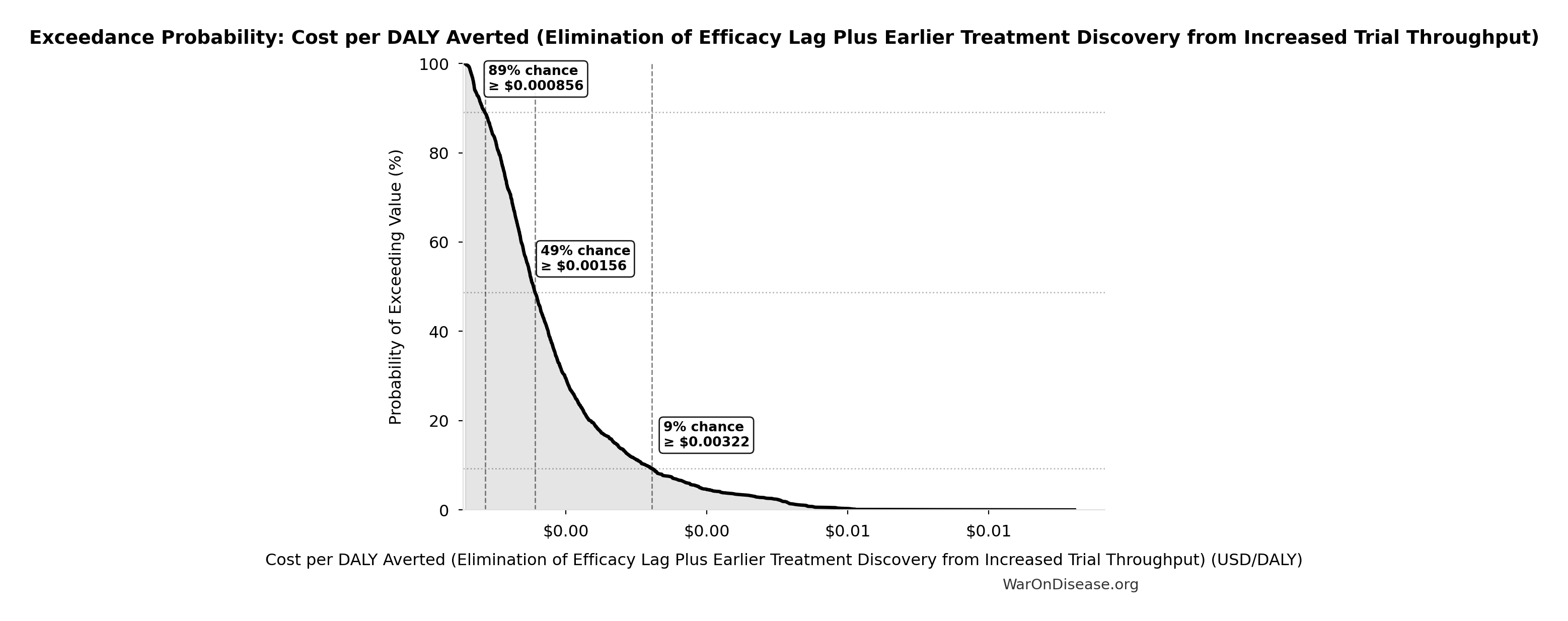
| Median (50th percentile) | $0.00156 |
| Standard Deviation | $0.00109 |
| 90% Range (5th-95th percentile) | [$0.000715, $0.00412] |
The histogram shows the distribution of Cost per DALY Averted (Elimination of Efficacy Lag Plus Earlier Treatment Discovery from Increased Trial Throughput) across 10,000 Monte Carlo simulations. The CDF (right) shows the probability of the outcome exceeding any given value, which is useful for risk assessment.
Exceedance Probability
This exceedance probability chart shows the likelihood that Cost per DALY Averted (Elimination of Efficacy Lag Plus Earlier Treatment Discovery from Increased Trial Throughput) will exceed any given threshold. Higher curves indicate more favorable outcomes with greater certainty.
Treaty ROI - Elimination of Efficacy Lag Plus Earlier Treatment Discovery from Increased Trial Throughput: 84.8M:1
Note📊 Details
Treaty ROI from elimination of efficacy lag plus earlier treatment discovery from increased trial throughput. Total one-time benefit divided by campaign cost. This is the primary ROI estimate for total health benefits.
Inputs:
- Total Economic Benefit from Elimination of Efficacy Lag Plus Earlier Treatment Discovery from Higher Trial Throughput 🔢: $84.8 quadrillion
- Total 1% Treaty Campaign Cost 🔢: $1B
\[ \begin{gathered} ROI_{max} \\ = \frac{Value_{max}}{Cost_{campaign}} \\ = \frac{\$84800T}{\$1B} \\ = 84.8M \end{gathered} \] where: \[ \begin{gathered} Value_{max} \\ = DALYs_{max} \times Value_{QALY} \\ = 565B \times \$150K \\ = \$84800T \end{gathered} \] where: \[ \begin{gathered} DALYs_{max} \\ = DALYs_{global,ann} \times Pct_{avoid,DALY} \times T_{accel,max} \\ = 2.88B \times 92.6\% \times 212 \\ = 565B \end{gathered} \] where: \[ T_{accel,max} = T_{accel} + T_{lag} = 204 + 8.2 = 212 \] where: \[ \begin{gathered} T_{accel} \\ = T_{first,SQ} \times \left(1 - \frac{1}{k_{capacity}}\right) \\ = 222 \times \left(1 - \frac{1}{12.3}\right) \\ = 204 \end{gathered} \] where: \[ \begin{gathered} T_{first,SQ} \\ = T_{queue,SQ} \times 0.5 \\ = 443 \times 0.5 \\ = 222 \end{gathered} \] where: \[ \begin{gathered} T_{queue,SQ} \\ = \frac{N_{untreated}}{Treatments_{new,ann}} \\ = \frac{6{,}650}{15} \\ = 443 \end{gathered} \] where: \[ \begin{gathered} N_{untreated} \\ = N_{rare} \times 0.95 \\ = 7{,}000 \times 0.95 \\ = 6{,}650 \end{gathered} \] where: \[ \begin{gathered} k_{capacity} \\ = \frac{N_{fundable,dFDA}}{Slots_{curr}} \\ = \frac{23.4M}{1.9M} \\ = 12.3 \end{gathered} \] where: \[ \begin{gathered} N_{fundable,dFDA} \\ = \frac{Subsidies_{dFDA,ann}}{Cost_{pragmatic,pt}} \\ = \frac{\$21.8B}{\$929} \\ = 23.4M \end{gathered} \] where: \[ \begin{gathered} Subsidies_{dFDA,ann} \\ = Funding_{dFDA,ann} - OPEX_{dFDA} \\ = \$21.8B - \$40M \\ = \$21.8B \end{gathered} \] where: \[ \begin{gathered} OPEX_{dFDA} \\ = Cost_{platform} + Cost_{staff} + Cost_{infra} \\ + Cost_{regulatory} + Cost_{community} \\ = \$15M + \$10M + \$8M + \$5M + \$2M \\ = \$40M \end{gathered} \] where: \[ \begin{gathered} Cost_{campaign} \\ = Budget_{viral,base} + Budget_{lobby,treaty} \\ + Budget_{reserve} \\ = \$250M + \$650M + \$100M \\ = \$1B \end{gathered} \] ~ Medium confidence
Sensitivity Analysis
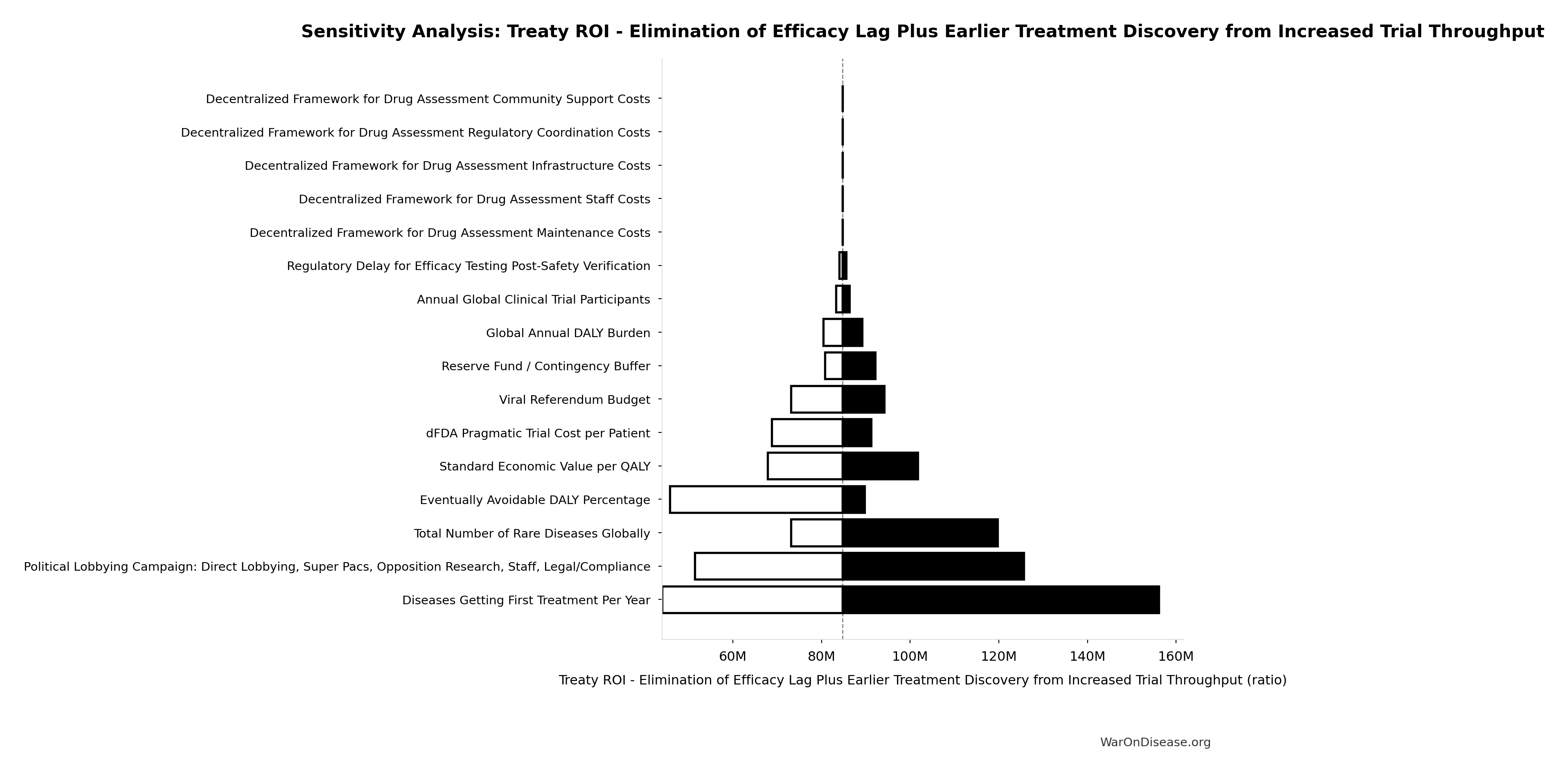
Sensitivity Indices for Treaty ROI - Elimination of Efficacy Lag Plus Earlier Treatment Discovery from Increased Trial Throughput
Regression-based sensitivity showing which inputs explain the most variance in the output.
| Input Parameter | Sensitivity Coefficient | Interpretation |
|---|---|---|
| Total 1% Treaty Campaign Cost (USD) | -0.7930 | Strong driver |
| Total Economic Benefit from Elimination of Efficacy Lag Plus Earlier Treatment Discovery from Higher Trial Throughput (USD) | 0.3364 | Moderate driver |
Interpretation: Standardized coefficients show the change in output (in SD units) per 1 SD change in input. Values near ±1 indicate strong influence; values exceeding ±1 may occur with correlated inputs.
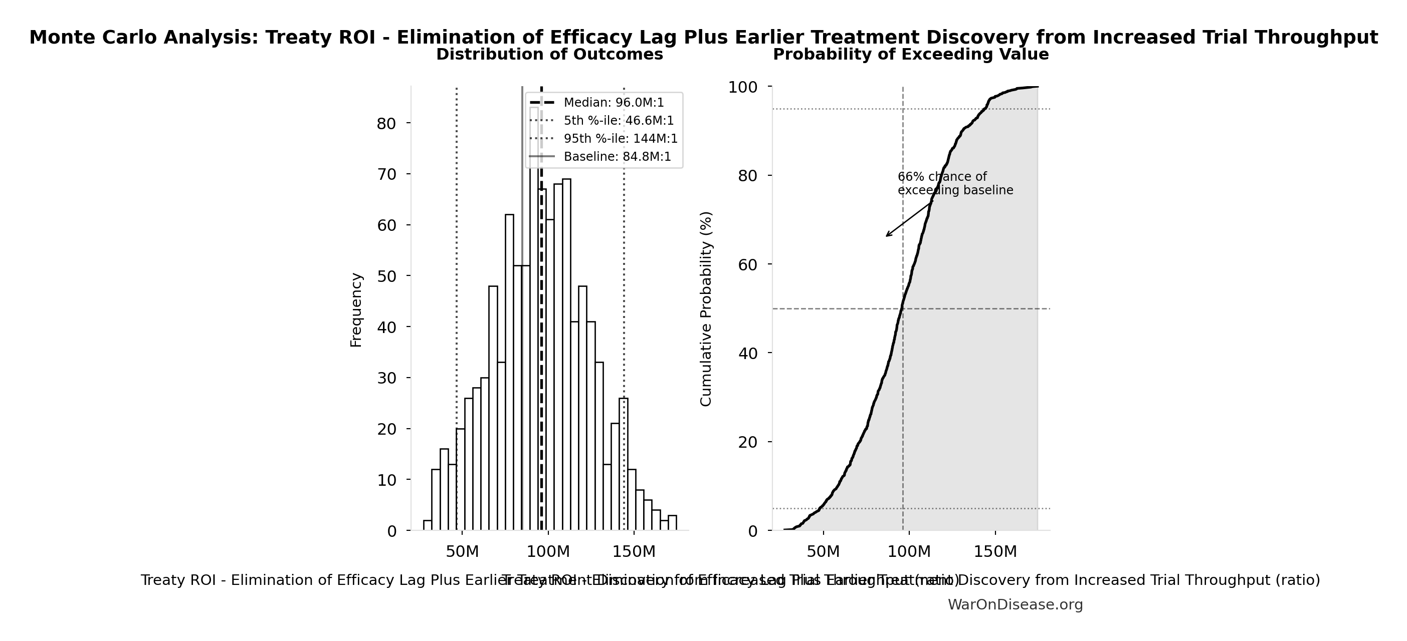
Monte Carlo Distribution
Simulation Results Summary: Treaty ROI - Elimination of Efficacy Lag Plus Earlier Treatment Discovery from Increased Trial Throughput
| Statistic | Value |
|---|---|
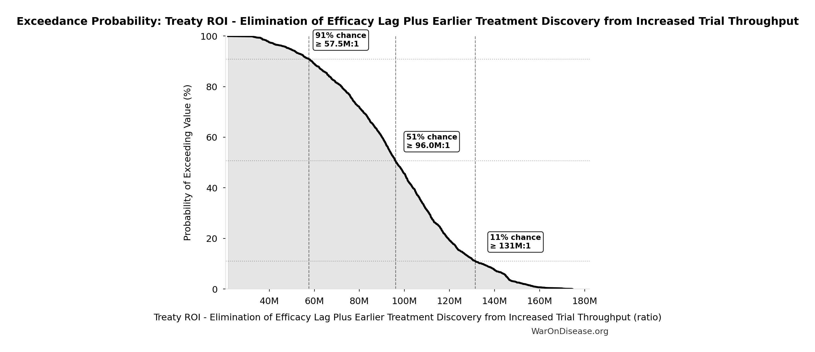
| Baseline (deterministic) | 84.8M:1 |
| Mean (expected value) | 95.1M:1 |
| Median (50th percentile) | 96.0M:1 |
| Standard Deviation | 28.1M:1 |
| 90% Range (5th-95th percentile) | [46.6M:1, 144M:1] |
The histogram shows the distribution of Treaty ROI - Elimination of Efficacy Lag Plus Earlier Treatment Discovery from Increased Trial Throughput across 10,000 Monte Carlo simulations. The CDF (right) shows the probability of the outcome exceeding any given value, which is useful for risk assessment.
Exceedance Probability
This exceedance probability chart shows the likelihood that Treaty ROI - Elimination of Efficacy Lag Plus Earlier Treatment Discovery from Increased Trial Throughput will exceed any given threshold. Higher curves indicate more favorable outcomes with greater certainty.
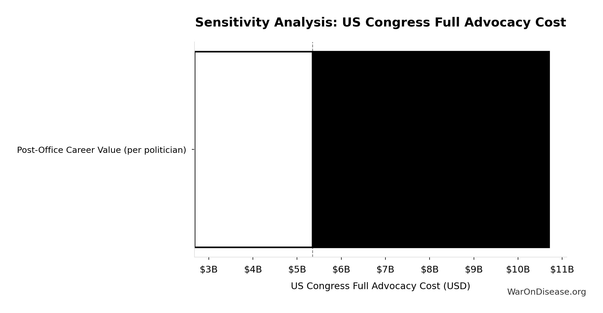
US Congress Full Advocacy Cost: $5.35B
Note📊 Details
Upper-bound advocacy cost to match career incentives for all 535 members of Congress
Inputs:
- US Congress Members: 535 members
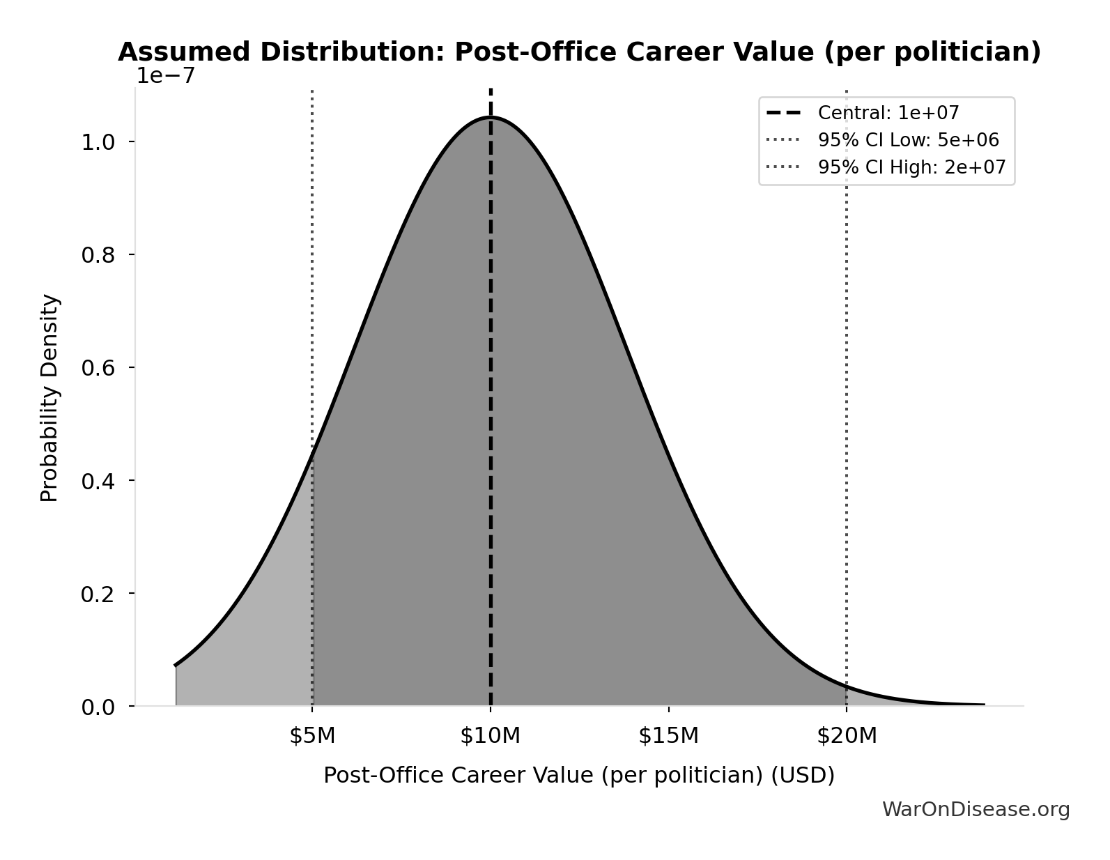
- Post-Office Career Value (per politician) 📊: $10M (95% CI: $5M - $20M)
\[ \begin{gathered} Cost_{US,congress} \\ = N_{congress} \times V_{post-office} \\ = 535 \times \$10M \\ = \$5.35B \end{gathered} \]
~ Medium confidence
Sensitivity Analysis
US Political Reform Investment (Total): $25.5B
Note📊 Details
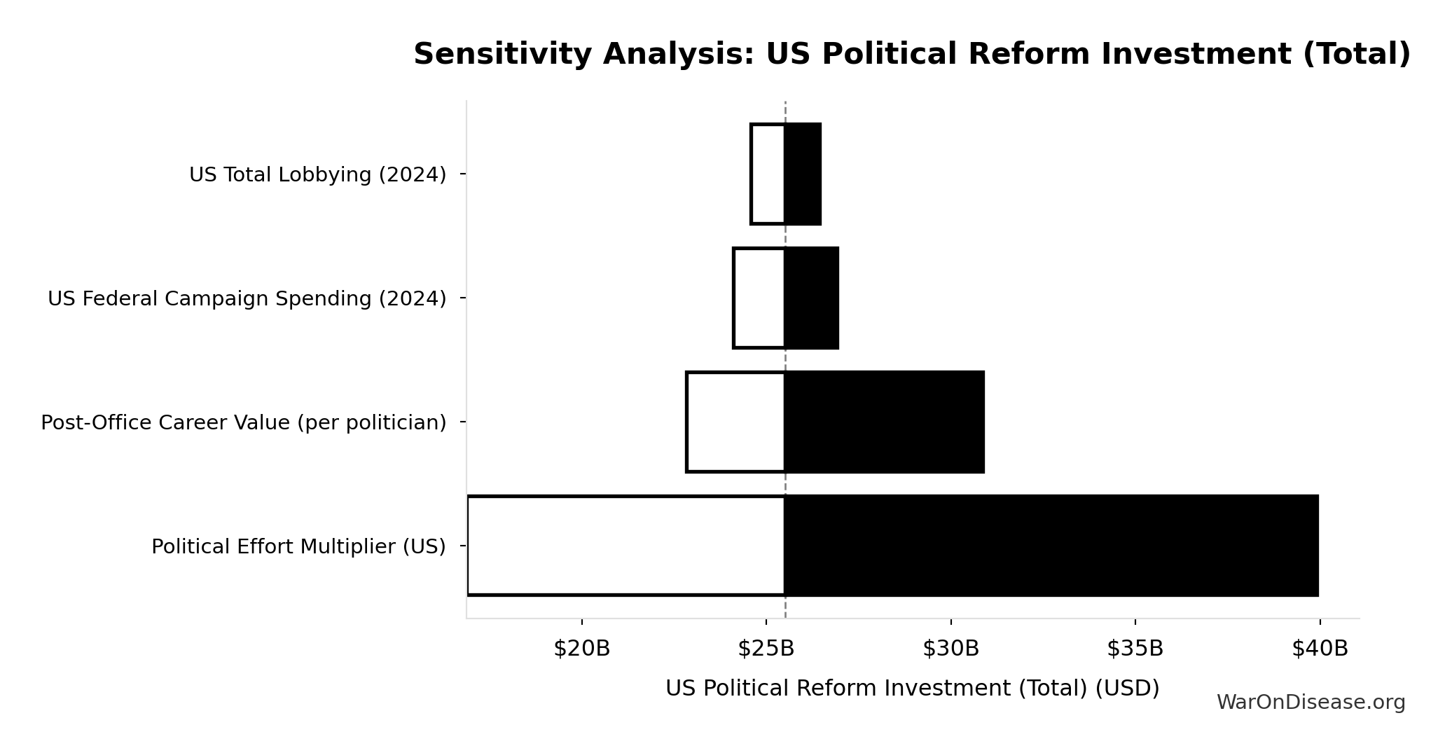
Total upper-bound investment for US political reform: (campaign spending + 2 years lobbying) × effort multiplier + Congress career advocacy. Represents cost to achieve democratic parity with incumbent interests.
Inputs:
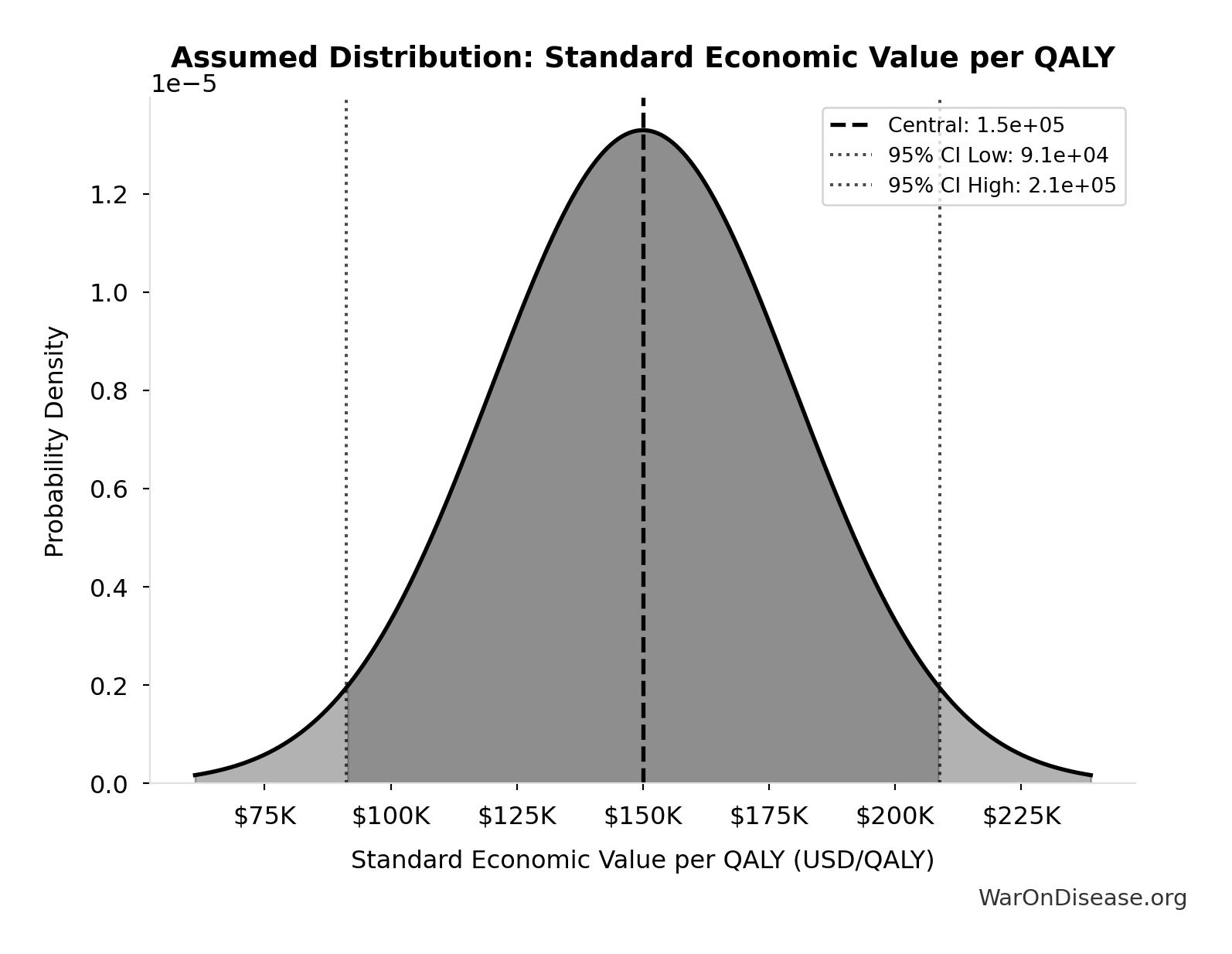
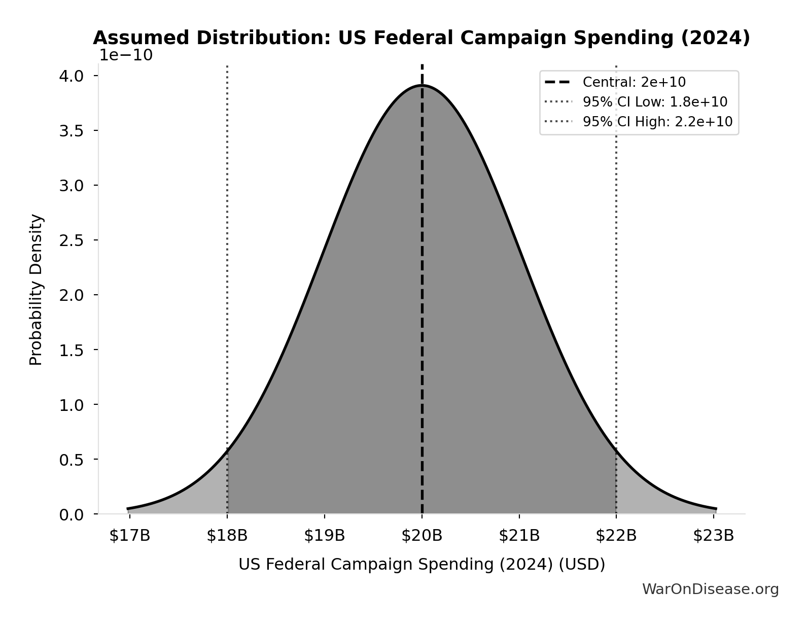
- US Federal Campaign Spending (2024) 📊: $20B (95% CI: $18B - $22B)
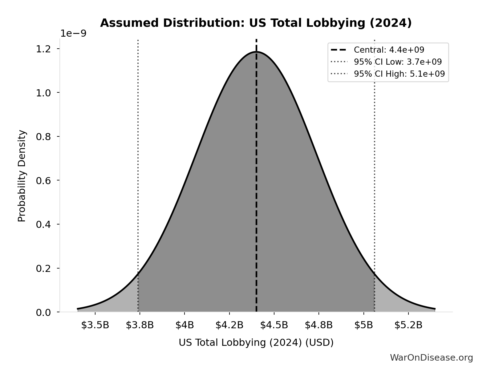
- US Total Lobbying (2024) 📊: $4.4B (95% CI: $3.74B - $5.06B)
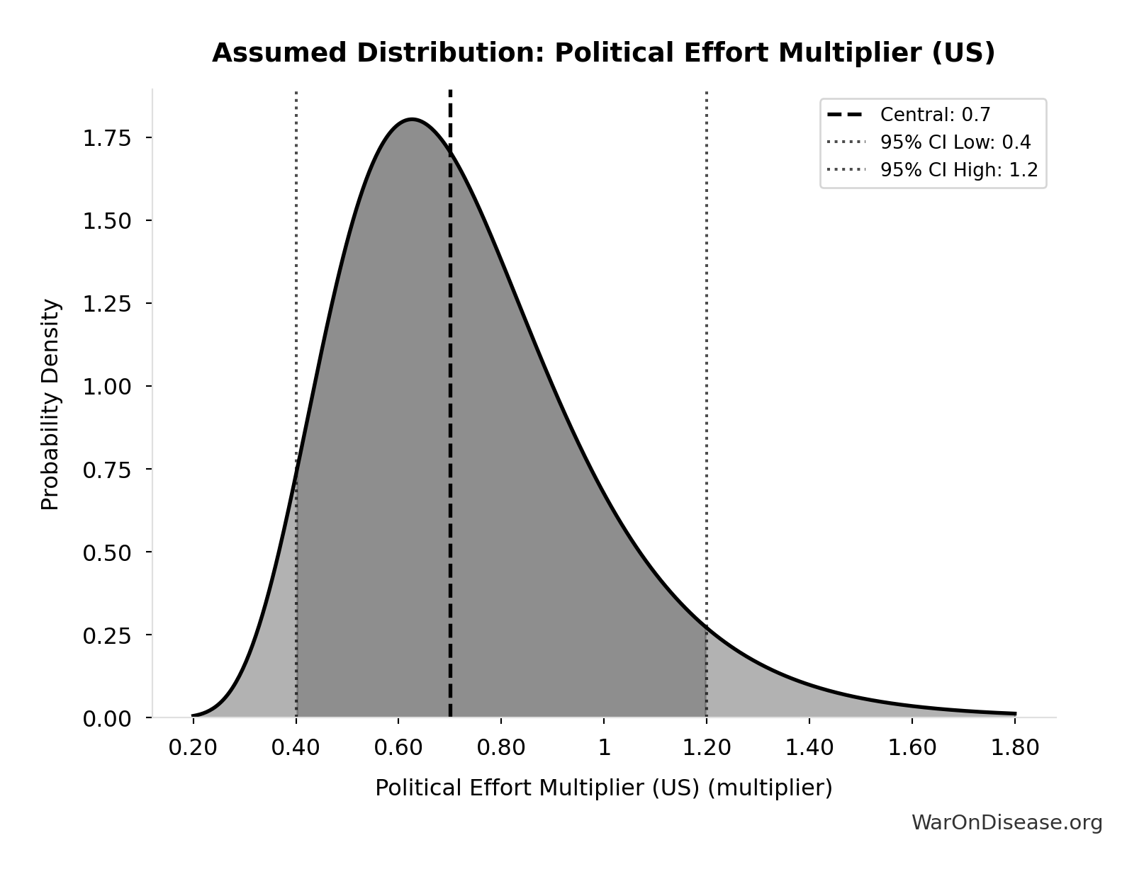
- Political Effort Multiplier (US): 0.7x (95% CI: 0.4x - 1.2x)
- US Congress Full Advocacy Cost 🔢: $5.35B
\[ \begin{gathered} Cost_{US,total} \\ = (Cost_{campaign} \\ + Cost_{lobby} \times 2) \times \mu_{effort} + Cost_{career} \end{gathered} \]
? Low confidence
Sensitivity Analysis
Sensitivity Indices for US Political Reform Investment (Total)
Regression-based sensitivity showing which inputs explain the most variance in the output.
| Input Parameter | Sensitivity Coefficient | Interpretation |
|---|---|---|
| Political Effort Multiplier (US) (multiplier) | 1.0000 | Strong driver |
Interpretation: Standardized coefficients show the change in output (in SD units) per 1 SD change in input. Values near ±1 indicate strong influence; values exceeding ±1 may occur with correlated inputs.
Monte Carlo Distribution
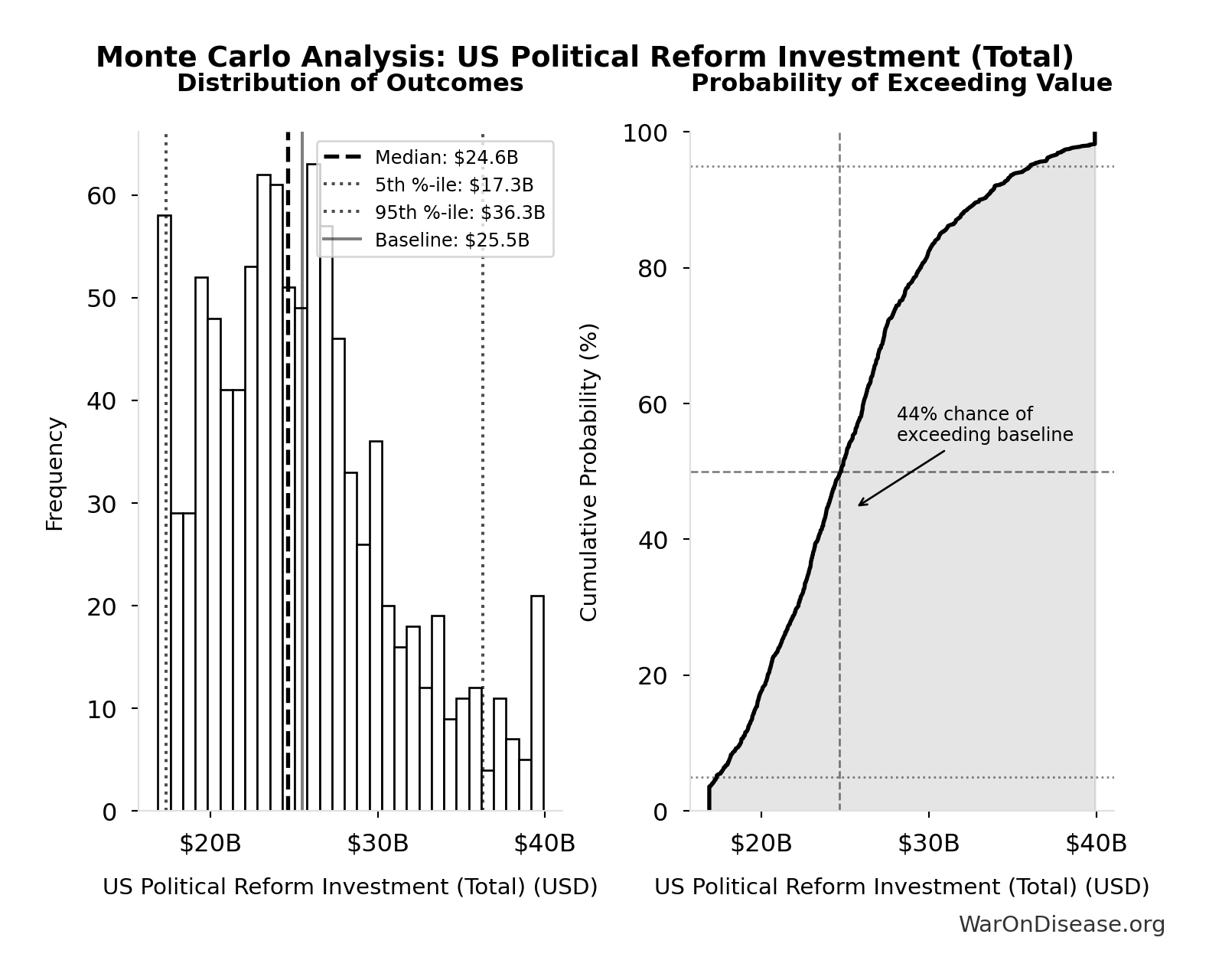
Simulation Results Summary: US Political Reform Investment (Total)
| Statistic | Value |
|---|---|
| Baseline (deterministic) | $25.5B |
| Mean (expected value) | $25.4B |
| Median (50th percentile) | $24.6B |
| Standard Deviation | $5.54B |
| 90% Range (5th-95th percentile) | [$17.3B, $36.3B] |
The histogram shows the distribution of US Political Reform Investment (Total) across 10,000 Monte Carlo simulations. The CDF (right) shows the probability of the outcome exceeding any given value, which is useful for risk assessment.
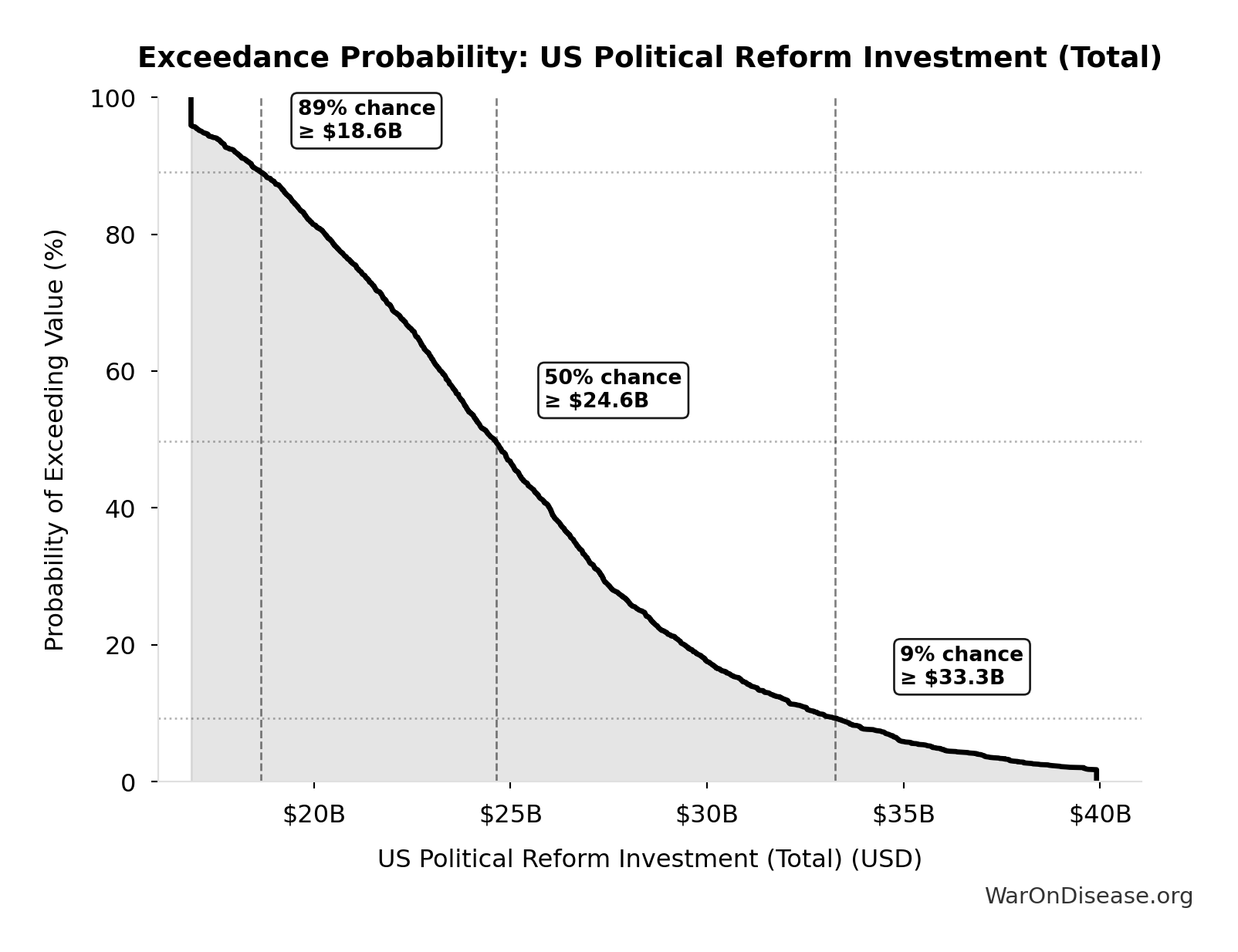
Exceedance Probability
This exceedance probability chart shows the likelihood that US Political Reform Investment (Total) will exceed any given threshold. Higher curves indicate more favorable outcomes with greater certainty.
Global Patients Willing to Participate in Clinical Trials: 1.08 billion people
Note📊 Details
Global chronic disease patients willing to participate in trials (2.4B × 44.8%)
Inputs:
- Global Population with Chronic Diseases 📊: 2.4 billion people (95% CI: 2 billion people - 2.8 billion people)
- Patient Willingness to Participate in Clinical Trials 📊: 44.8% (95% CI: 40% - 50%)
\[ \begin{gathered} N_{willing} \\ = N_{patients} \times Pct_{willing} \\ = 2.4B \times 44.8\% \\ = 1.08B \end{gathered} \]
~ Medium confidence
Sensitivity Analysis
Sensitivity Indices for Global Patients Willing to Participate in Clinical Trials
Regression-based sensitivity showing which inputs explain the most variance in the output.
| Input Parameter | Sensitivity Coefficient | Interpretation |
|---|---|---|
| Global Population with Chronic Diseases (people) | 1.1065 | Strong driver |
| Patient Willingness to Participate in Clinical Trials (percentage) | -0.1072 | Weak driver |
Interpretation: Standardized coefficients show the change in output (in SD units) per 1 SD change in input. Values near ±1 indicate strong influence; values exceeding ±1 may occur with correlated inputs.
Monte Carlo Distribution
Simulation Results Summary: Global Patients Willing to Participate in Clinical Trials
| Statistic | Value |
|---|---|
| Baseline (deterministic) | 1.08 billion |
| Mean (expected value) | 1.08 billion |
| Median (50th percentile) | 1.07 billion |
| Standard Deviation | 145 million |
| 90% Range (5th-95th percentile) | [843 million, 1.34 billion] |
The histogram shows the distribution of Global Patients Willing to Participate in Clinical Trials across 10,000 Monte Carlo simulations. The CDF (right) shows the probability of the outcome exceeding any given value, which is useful for risk assessment.
Exceedance Probability
This exceedance probability chart shows the likelihood that Global Patients Willing to Participate in Clinical Trials will exceed any given threshold. Higher curves indicate more favorable outcomes with greater certainty.
Wishonia Disease Cure Fraction (20yr, Full Implementation): 100%
Note📊 Details
Wishonia disease-cure fraction over 20 years under full implementation. Uses full trial-capacity scaling and applies an upper bound of 100% of untreated disease classes.
Inputs:
- Diseases Getting First Treatment Per Year 📊: 15 diseases/year (95% CI: 8 diseases/year - 30 diseases/year)
- Trial Capacity Multiplier 🔢: 12.3x
- Wishonia Military Reallocation Physical Max Share 🔢: 87.6%
- Maximum Trial Capacity Multiplier (Physical Limit) 🔢: 566x
- Diseases Without Effective Treatment 🔢: 6.65 thousand diseases
\[ \begin{gathered} f_{cure,20,wish} \\ = \min\left(1,\frac{Treatments_{new,ann}\cdot k_{capacity,wish}\cdot 20}{D_{untreated}}\right) \end{gathered} \]
✓ High confidence
Wishonia Trajectory Average Income at Year 20: $1.16M
Note📊 Details
Average income (GDP per capita) at year 20 under the Wishonia Trajectory.
Inputs:
- Wishonia Trajectory GDP at Year 20 🔢: $10.7 quadrillion
- Global Population 2045 (Projected) 📊: 9.2 billion of people
\[ \bar{y}_{wish,20} = \frac{GDP_{wish,20}}{Pop_{2045}} \]
✓ High confidence
Sensitivity Analysis
Sensitivity Indices for Wishonia Trajectory Average Income at Year 20
Regression-based sensitivity showing which inputs explain the most variance in the output.
| Input Parameter | Sensitivity Coefficient | Interpretation |
|---|---|---|
| Wishonia Trajectory GDP at Year 20 (USD) | 1.0000 | Strong driver |
Interpretation: Standardized coefficients show the change in output (in SD units) per 1 SD change in input. Values near ±1 indicate strong influence; values exceeding ±1 may occur with correlated inputs.
Monte Carlo Distribution
Simulation Results Summary: Wishonia Trajectory Average Income at Year 20
| Statistic | Value |
|---|---|
| Baseline (deterministic) | $1.16M |
| Mean (expected value) | $1.87M |
| Median (50th percentile) | $1.15M |
| Standard Deviation | $1.98M |
| 90% Range (5th-95th percentile) | [$395K, $6.22M] |
The histogram shows the distribution of Wishonia Trajectory Average Income at Year 20 across 10,000 Monte Carlo simulations. The CDF (right) shows the probability of the outcome exceeding any given value, which is useful for risk assessment.
Exceedance Probability
This exceedance probability chart shows the likelihood that Wishonia Trajectory Average Income at Year 20 will exceed any given threshold. Higher curves indicate more favorable outcomes with greater certainty.
Wishonia Trajectory vs Current Trajectory GDP Multiplier (Year 20): 56.7x
Note📊 Details
Wishonia Trajectory GDP at year 20 as a multiple of current trajectory GDP at year 20.
Inputs:
- Wishonia Trajectory GDP at Year 20 🔢: $10.7 quadrillion
- Current Trajectory GDP at Year 20 🔢: $188T
\[ \begin{gathered} k_{wish:base,20} \\ = \frac{GDP_{wish,20}}{GDP_{base,20}} \\ = \frac{\$10700T}{\$188T} \\ = 56.7 \end{gathered} \] where: \[ GDP_{wish,20}=GDP_0(1+g_{ramp})^3(1+g_{full})^{17} \] where: \[ s_{mil,max} = Cut_{WW2} = 87.6\% = 87.6\% \] where: \[ \begin{gathered} Cut_{WW2} \\ = 1 - \frac{Spending_{US,1947}}{Spending_{US,1945}} \\ = 1 - \frac{\$176B}{\$1.42T} \\ = 87.6\% \end{gathered} \] where: \[ \begin{gathered} f_{cure,20,wish} \\ = \min\left(1,\frac{Treatments_{new,ann}\cdot k_{capacity,wish}\cdot 20}{D_{untreated}}\right) \end{gathered} \] where: \[ \begin{gathered} k_{capacity} \\ = \frac{N_{fundable,dFDA}}{Slots_{curr}} \\ = \frac{23.4M}{1.9M} \\ = 12.3 \end{gathered} \] where: \[ \begin{gathered} N_{fundable,dFDA} \\ = \frac{Subsidies_{dFDA,ann}}{Cost_{pragmatic,pt}} \\ = \frac{\$21.8B}{\$929} \\ = 23.4M \end{gathered} \] where: \[ \begin{gathered} Subsidies_{dFDA,ann} \\ = Funding_{dFDA,ann} - OPEX_{dFDA} \\ = \$21.8B - \$40M \\ = \$21.8B \end{gathered} \] where: \[ \begin{gathered} OPEX_{dFDA} \\ = Cost_{platform} + Cost_{staff} + Cost_{infra} \\ + Cost_{regulatory} + Cost_{community} \\ = \$15M + \$10M + \$8M + \$5M + \$2M \\ = \$40M \end{gathered} \] where: \[ \begin{gathered} k_{capacity,max} \\ = \frac{N_{willing}}{Slots_{curr}} \\ = \frac{1.08B}{1.9M} \\ = 566 \end{gathered} \] where: \[ \begin{gathered} N_{willing} \\ = N_{patients} \times Pct_{willing} \\ = 2.4B \times 44.8\% \\ = 1.08B \end{gathered} \] where: \[ \begin{gathered} N_{untreated} \\ = N_{rare} \times 0.95 \\ = 7{,}000 \times 0.95 \\ = 6{,}650 \end{gathered} \] where: \[ GDP_{base,20} = GDP_0(1+g_{base})^{20} \] ✓ High confidence
Sensitivity Analysis
Sensitivity Indices for Wishonia Trajectory vs Current Trajectory GDP Multiplier (Year 20)
Regression-based sensitivity showing which inputs explain the most variance in the output.
| Input Parameter | Sensitivity Coefficient | Interpretation |
|---|---|---|
| Wishonia Trajectory GDP at Year 20 (USD) | 1.0000 | Strong driver |
| Current Trajectory GDP at Year 20 (USD) | 0.0000 | Minimal effect |
Interpretation: Standardized coefficients show the change in output (in SD units) per 1 SD change in input. Values near ±1 indicate strong influence; values exceeding ±1 may occur with correlated inputs.
Monte Carlo Distribution
Simulation Results Summary: Wishonia Trajectory vs Current Trajectory GDP Multiplier (Year 20)
| Statistic | Value |
|---|---|
| Baseline (deterministic) | 56.7x |
| Mean (expected value) | 91.5x |
| Median (50th percentile) | 56.2x |
| Standard Deviation | 96.6x |
| 90% Range (5th-95th percentile) | [19.3x, 304x] |
The histogram shows the distribution of Wishonia Trajectory vs Current Trajectory GDP Multiplier (Year 20) across 10,000 Monte Carlo simulations. The CDF (right) shows the probability of the outcome exceeding any given value, which is useful for risk assessment.
Exceedance Probability
This exceedance probability chart shows the likelihood that Wishonia Trajectory vs Current Trajectory GDP Multiplier (Year 20) will exceed any given threshold. Higher curves indicate more favorable outcomes with greater certainty.
Wishonia Trajectory GDP at Year 20: $10.7 quadrillion
Note📊 Details
Projected global GDP at year 20 under the Wishonia Trajectory. Model applies all Wishonia policy channels and redirects the full Political Dysfunction Tax non-health opportunity pool to highest-marginal-value uses. Health recovery is modeled separately through disease burden removal to avoid overlap. Military and non-health reallocation effects are ramped at 50% intensity for the first 3 years, then 100% for years 4-20, reflecting implementation lag. Military reallocation uses a physically demonstrated upper bound (post-WW2 demobilization) rather than an arbitrary policy cap.
Inputs:
- Global GDP (2025) 📊: $115T
- Baseline Global GDP Growth Rate: 2.5%
- Wishonia Military Reallocation Physical Max Share 🔢: 87.6%
- GDP Growth Boost at 30% Military Reallocation: 5.5% (95% CI: 3.5% - 7.5%)
- R&D Spillover Multiplier: 2x (95% CI: 1.5x - 2.5x)
- Wishonia Disease Cure Fraction (20yr, Full Implementation) 🔢: 100%
- Disease Burden as % of GDP 📊: 13%
- Global Science Opportunity Cost 📊: $4T (95% CI: $2T - $10T)
- Global Lead Poisoning Cost 📊: $6T (95% CI: $4T - $8T)
- Global Migration Opportunity Cost 📊: $57T (95% CI: $57T - $170T)
- Economic Multiplier for Healthcare Investment 📊: 4.3x (95% CI: 3x - 6x)
- Economic Multiplier for Military Spending 📊: 0.6x (95% CI: 0.4x - 0.9x)
\[ GDP_{wish,20}=GDP_0(1+g_{ramp})^3(1+g_{full})^{17} \]
✓ High confidence
Sensitivity Analysis
Sensitivity Indices for Wishonia Trajectory GDP at Year 20
Regression-based sensitivity showing which inputs explain the most variance in the output.
| Input Parameter | Sensitivity Coefficient | Interpretation |
|---|---|---|
| Economic Multiplier for Healthcare Investment (x) | -1.7151 | Strong driver |
| R&D Spillover Multiplier (x) | 1.3750 | Strong driver |
| Global Science Opportunity Cost (USD) | 0.9398 | Strong driver |
| Global Migration Opportunity Cost (USD) | 0.6829 | Strong driver |
| GDP Growth Boost at 30% Military Reallocation (rate) | -0.3425 | Moderate driver |
| Global Lead Poisoning Cost (USD) | 0.2431 | Weak driver |
| Economic Multiplier for Military Spending (x) | -0.1554 | Weak driver |
Interpretation: Standardized coefficients show the change in output (in SD units) per 1 SD change in input. Values near ±1 indicate strong influence; values exceeding ±1 may occur with correlated inputs.
Monte Carlo Distribution
Simulation Results Summary: Wishonia Trajectory GDP at Year 20
| Statistic | Value |
|---|---|
| Baseline (deterministic) | $10.7 quadrillion |
| Mean (expected value) | $17.2 quadrillion |
| Median (50th percentile) | $10.6 quadrillion |
| Standard Deviation | $18.2 quadrillion |
| 90% Range (5th-95th percentile) | [$3.64 quadrillion, $57.2 quadrillion] |
The histogram shows the distribution of Wishonia Trajectory GDP at Year 20 across 10,000 Monte Carlo simulations. The CDF (right) shows the probability of the outcome exceeding any given value, which is useful for risk assessment.
Exceedance Probability
This exceedance probability chart shows the likelihood that Wishonia Trajectory GDP at Year 20 will exceed any given threshold. Higher curves indicate more favorable outcomes with greater certainty.
External Data Sources
Parameters sourced from peer-reviewed publications, institutional databases, and authoritative reports.
Bed Nets Cost per DALY: $89
Note📊 Details
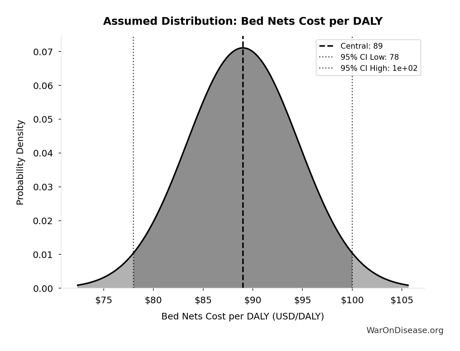
GiveWell cost per DALY for insecticide-treated bed nets (midpoint estimate, range $78-100). DALYs (Disability-Adjusted Life Years) measure disease burden by combining years of life lost and years lived with disability. Bed nets prevent malaria deaths and are considered a gold standard benchmark for cost-effective global health interventions - if an intervention costs less per DALY than bed nets, it’s exceptionally cost-effective. GiveWell synthesizes peer-reviewed academic research with transparent, rigorous methodology and extensive external expert review.
Source:5
Uncertainty Range
Technical: 95% CI: [$78, $100] • Distribution: Normal
What this means: This estimate has moderate uncertainty. The true value likely falls between $78 and $100 (±12%). This represents a reasonable range that our Monte Carlo simulations account for when calculating overall uncertainty in the results.
The normal distribution means values cluster around the center with equal chances of being higher or lower.
Input Distribution
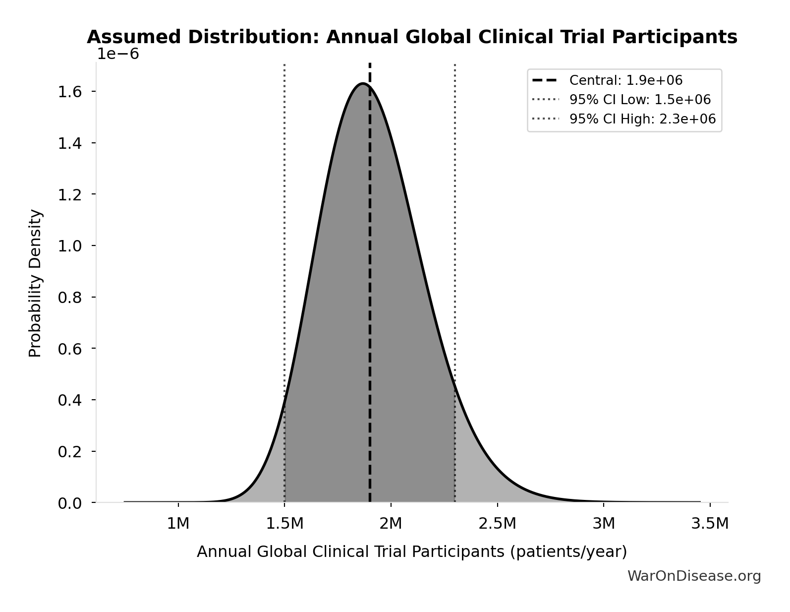
This chart shows the assumed probability distribution for this parameter. The shaded region represents the 95% confidence interval where we expect the true value to fall.
✓ High confidence • 📊 Peer-reviewed
Global Population with Chronic Diseases: 2.4 billion people
Note📊 Details
Global population with chronic diseases
Source:14
Uncertainty Range
Technical: 95% CI: [2 billion people, 2.8 billion people] • Distribution: Lognormal
What this means: This estimate has moderate uncertainty. The true value likely falls between 2 billion people and 2.8 billion people (±17%). This represents a reasonable range that our Monte Carlo simulations account for when calculating overall uncertainty in the results.
The lognormal distribution means values can’t go negative and have a longer tail toward higher values (common for costs and populations).
Input Distribution
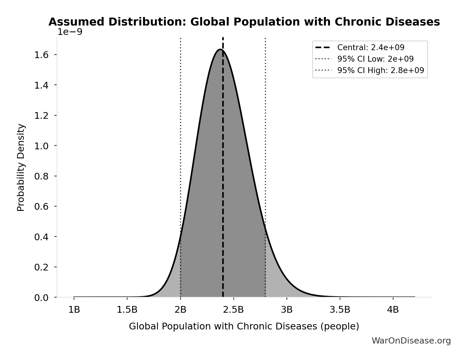
This chart shows the assumed probability distribution for this parameter. The shaded region represents the 95% confidence interval where we expect the true value to fall.
✓ High confidence
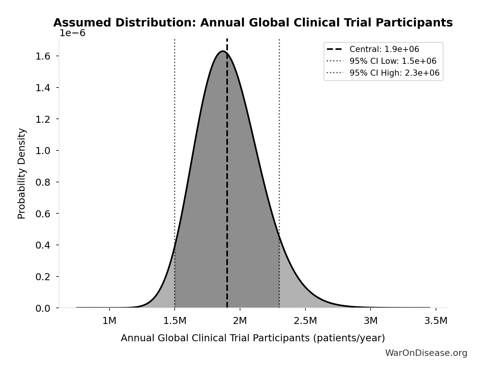
Annual Global Clinical Trial Participants: 1.9 million patients/year
Note📊 Details
Annual global clinical trial participants (IQVIA 2022: 1.9M post-COVID normalization)
Source:17
Uncertainty Range
Technical: 95% CI: [1.5 million patients/year, 2.3 million patients/year] • Distribution: Lognormal
What this means: This estimate has moderate uncertainty. The true value likely falls between 1.5 million patients/year and 2.3 million patients/year (±21%). This represents a reasonable range that our Monte Carlo simulations account for when calculating overall uncertainty in the results.
The lognormal distribution means values can’t go negative and have a longer tail toward higher values (common for costs and populations).
Input Distribution
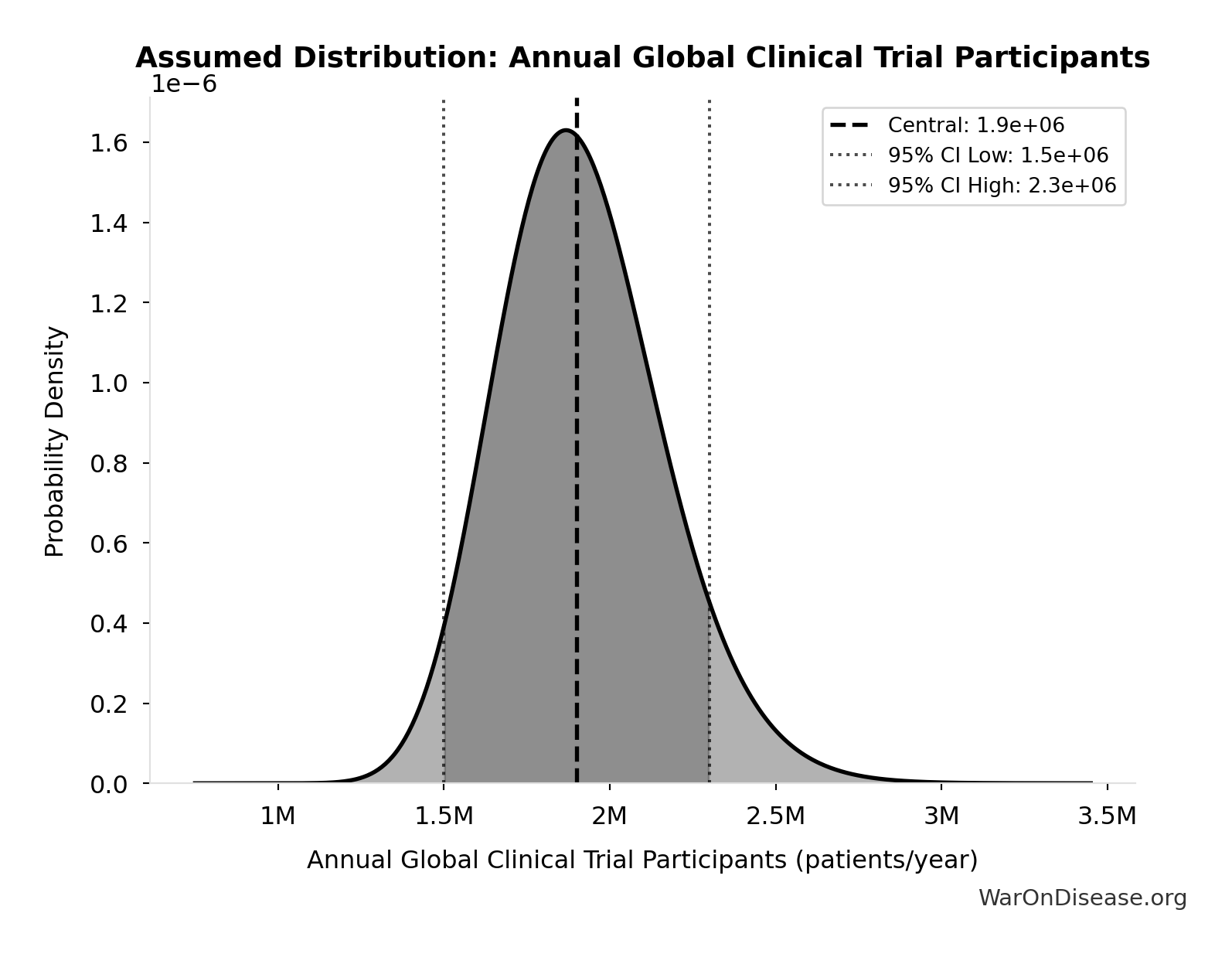
This chart shows the assumed probability distribution for this parameter. The shaded region represents the 95% confidence interval where we expect the true value to fall.
✓ High confidence
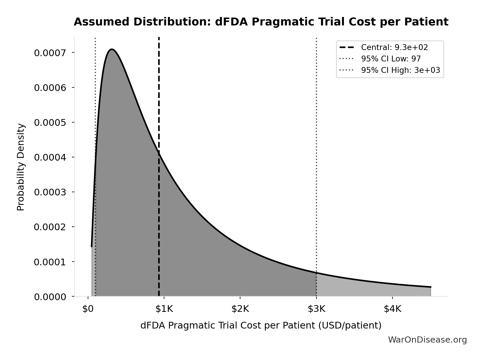
dFDA Pragmatic Trial Cost per Patient: $929
Note📊 Details
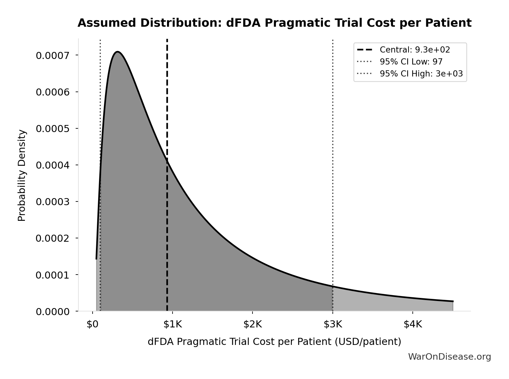
dFDA pragmatic trial cost per patient. Uses ADAPTABLE trial ($929) as DELIBERATELY CONSERVATIVE central estimate. Ramsberg & Platt (2018) reviewed 108 embedded pragmatic trials; 64 with cost data had median of only $97/patient - our estimate may overstate costs by 10x. Confidence interval spans meta-analysis median to complex chronic disease trials.
Source:1
Uncertainty Range
Technical: 95% CI: [$97, $3K] • Distribution: Lognormal
What this means: This estimate is highly uncertain. The true value likely falls between $97 and $3K (±156%). This represents a very wide range that our Monte Carlo simulations account for when calculating overall uncertainty in the results.
The lognormal distribution means values can’t go negative and have a longer tail toward higher values (common for costs and populations).
Input Distribution
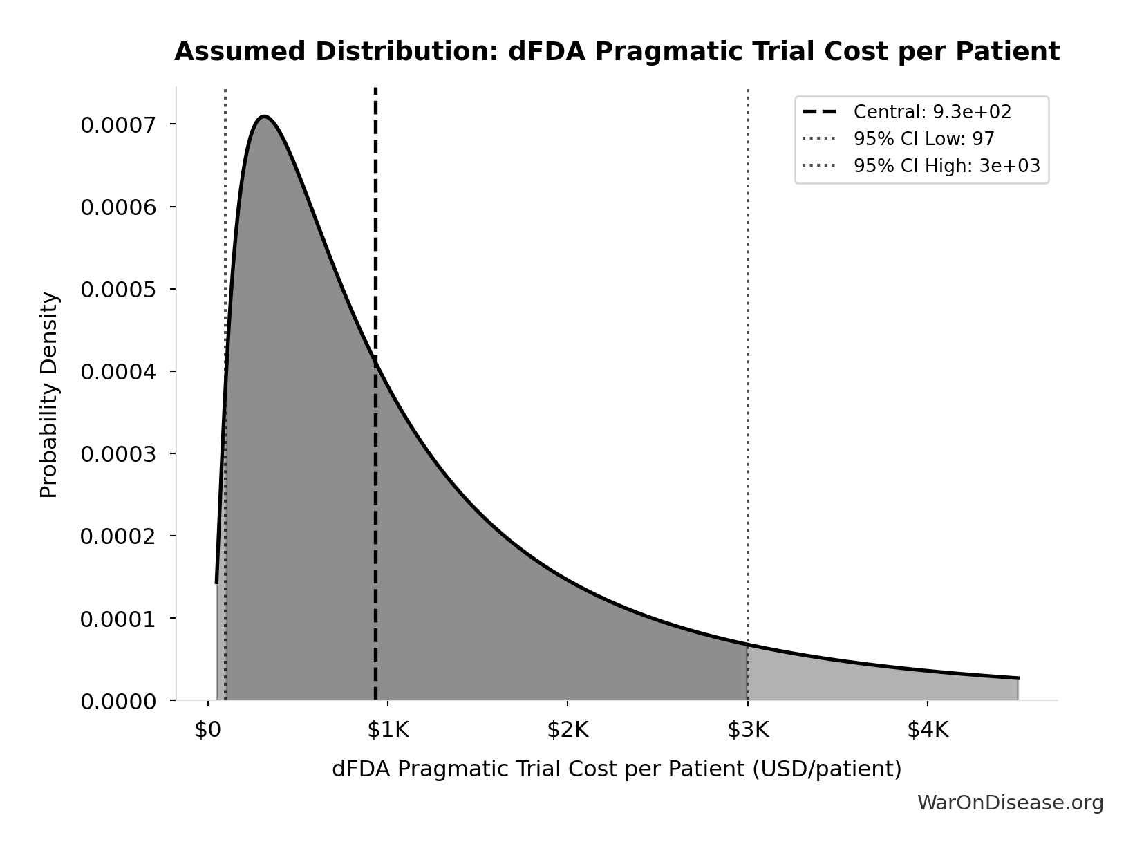
This chart shows the assumed probability distribution for this parameter. The shaded region represents the 95% confidence interval where we expect the true value to fall.
~ Medium confidence
Disease Burden as % of GDP: 13%
Note📊 Details
Fraction of GDP currently lost to disease (productivity losses + medical costs diverted from productive use). $5T productivity loss + $9.9T direct medical costs = $14.9T on $115T GDP = ~13%. As diseases are progressively cured, this drag is recovered as GDP growth. This is the missing factor that makes the treaty trajectory look like a singularity rather than a modest improvement.
Source:21
Uncertainty Range
Technical: Distribution: Fixed
✓ High confidence
Economic Multiplier for Healthcare Investment: 4.3x
Note📊 Details
Economic multiplier for healthcare investment (4.3x ROI). Literature range 3.0-6.0×.
Source:27
Uncertainty Range
Technical: 95% CI: [3x, 6x] • Distribution: Lognormal
What this means: There’s significant uncertainty here. The true value likely falls between 3x and 6x (±35%). This represents a wide range that our Monte Carlo simulations account for when calculating overall uncertainty in the results.
The lognormal distribution means values can’t go negative and have a longer tail toward higher values (common for costs and populations).
Input Distribution
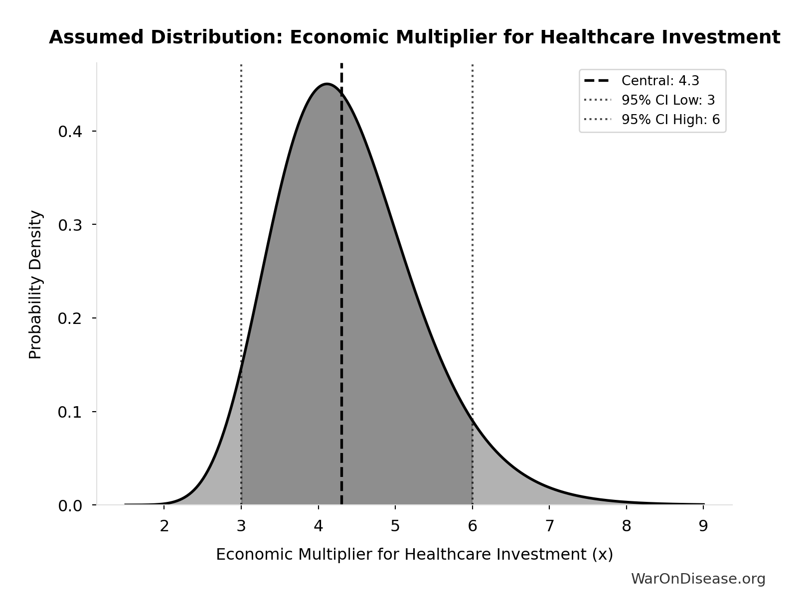
This chart shows the assumed probability distribution for this parameter. The shaded region represents the 95% confidence interval where we expect the true value to fall.
✓ High confidence
Economic Multiplier for Military Spending: 0.6x
Note📊 Details
Economic multiplier for military spending (0.6x ROI). Literature range 0.4-1.0×.
Source:29
Uncertainty Range
Technical: 95% CI: [0.4x, 0.9x] • Distribution: Lognormal
What this means: There’s significant uncertainty here. The true value likely falls between 0.4x and 0.9x (±42%). This represents a wide range that our Monte Carlo simulations account for when calculating overall uncertainty in the results.
The lognormal distribution means values can’t go negative and have a longer tail toward higher values (common for costs and populations).
Input Distribution
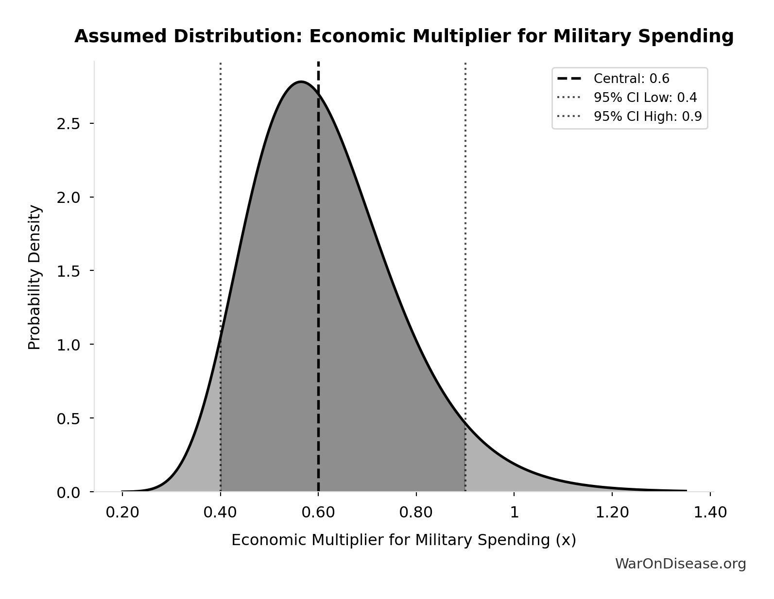
This chart shows the assumed probability distribution for this parameter. The shaded region represents the 95% confidence interval where we expect the true value to fall.
✓ High confidence
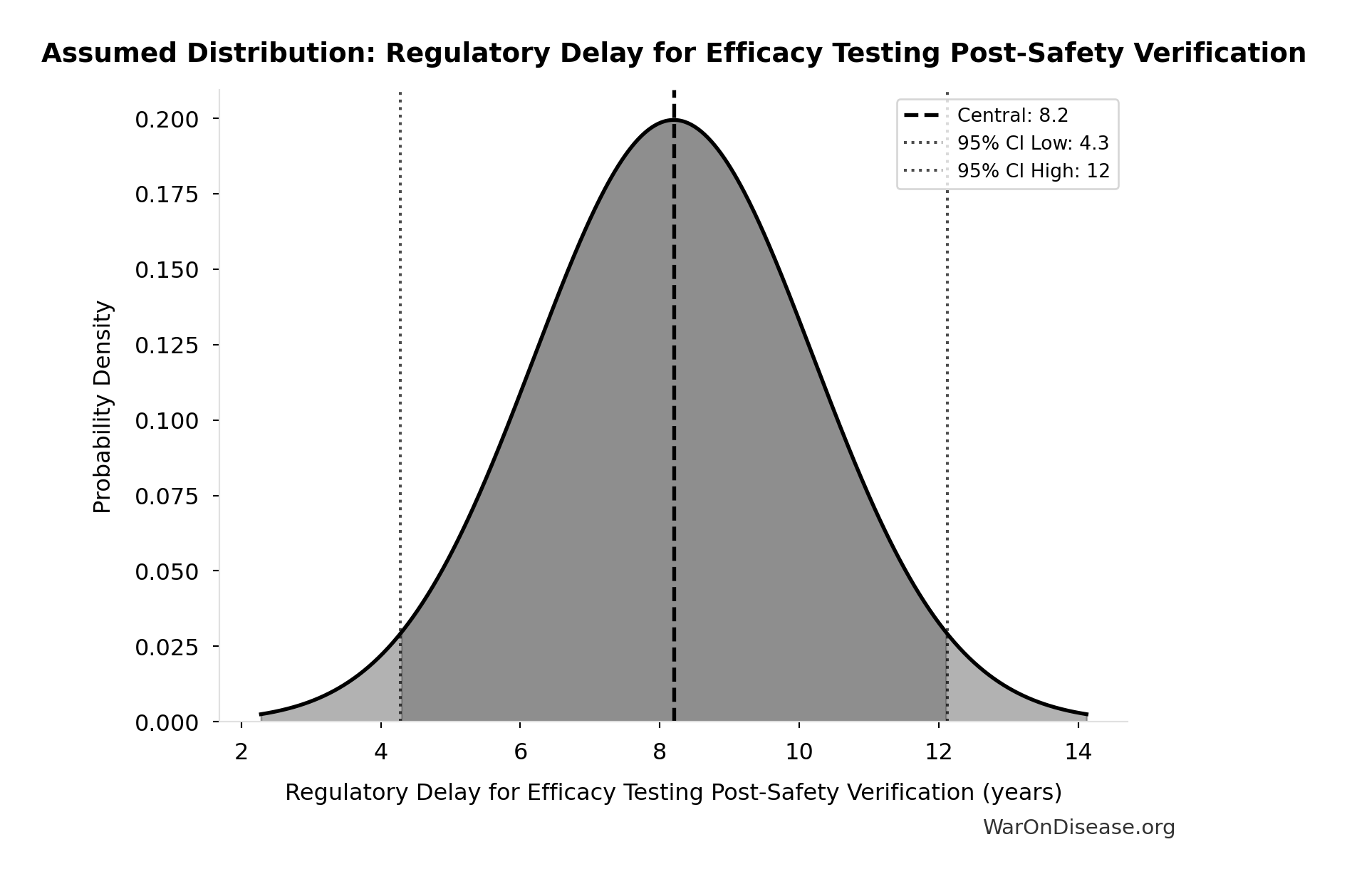
Regulatory Delay for Efficacy Testing Post-Safety Verification: 8.2 years
Note📊 Details
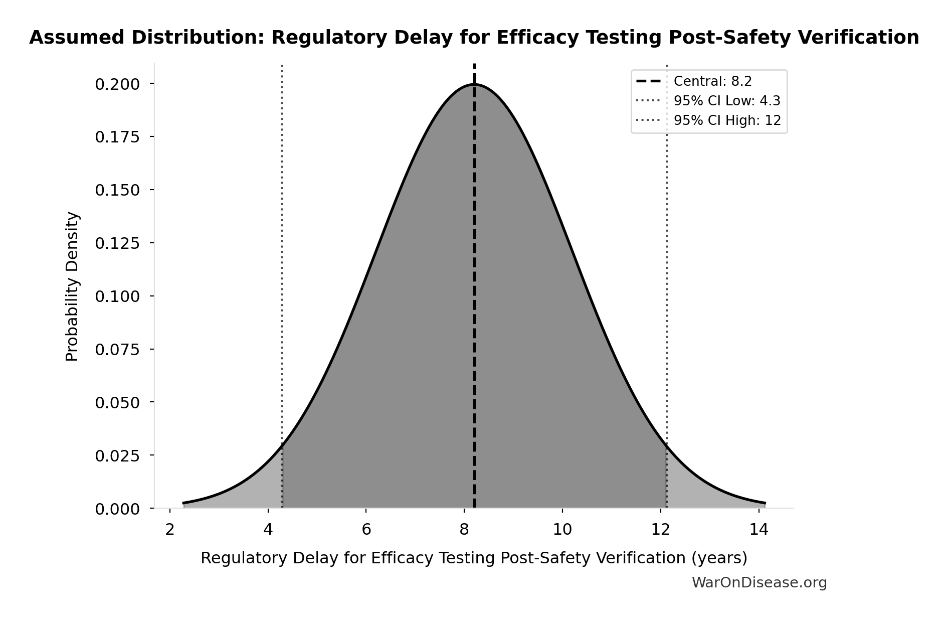
Regulatory delay for efficacy testing (Phase II/III) post-safety verification. Based on BIO 2021 industry survey. Note: This is for drugs that COMPLETE the pipeline - survivor bias means actual delay for any given disease may be longer if candidates fail and must restart.
Source:24
Uncertainty Range
Technical: Distribution: Normal (SE: 2 years)
Input Distribution
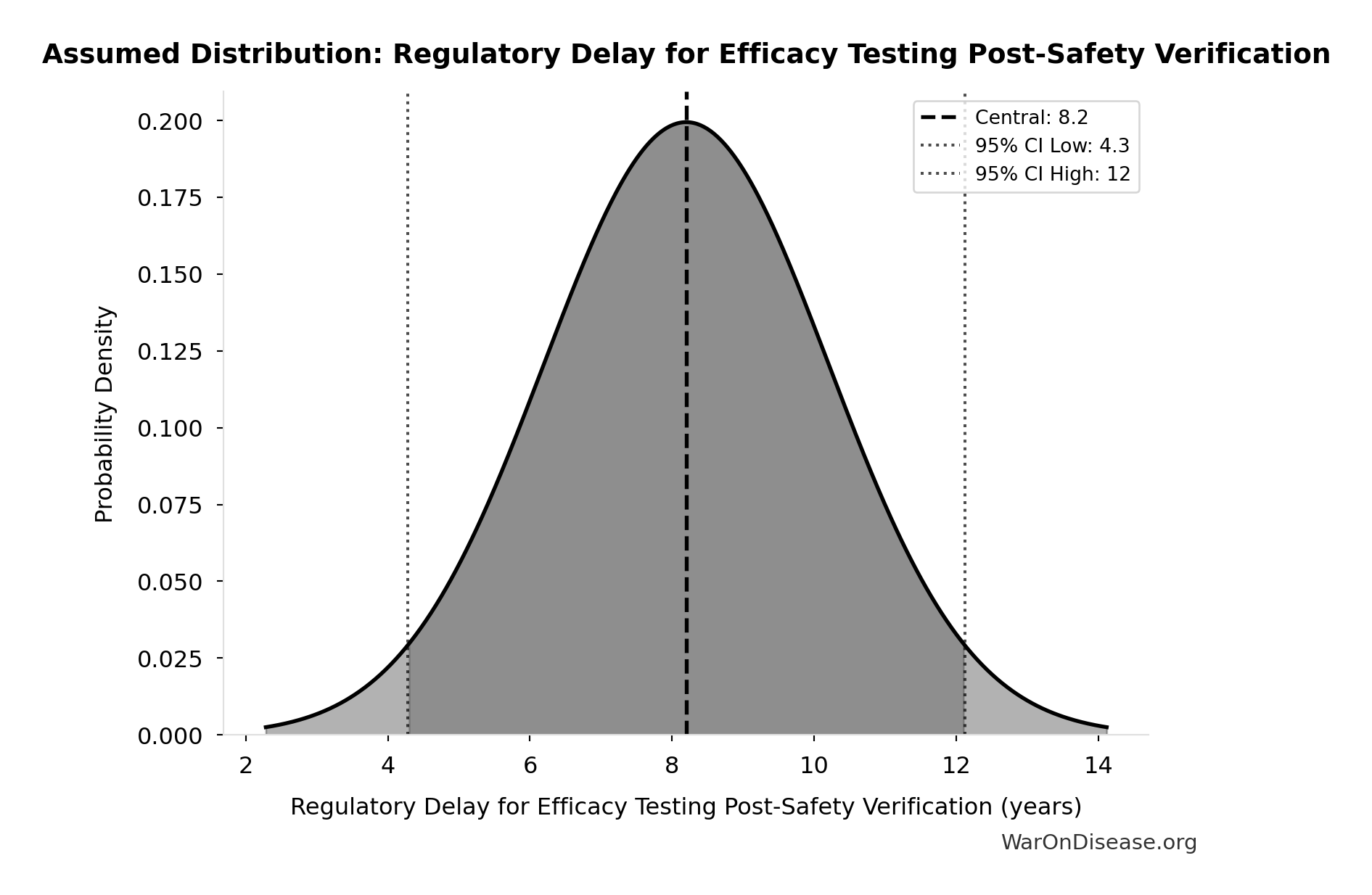
This chart shows the assumed probability distribution for this parameter. The shaded region represents the 95% confidence interval where we expect the true value to fall.
~ Medium confidence • 📊 Peer-reviewed • Updated 2021
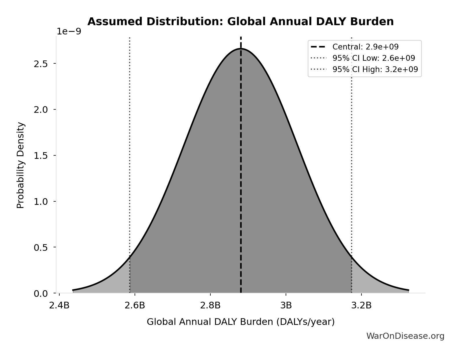
Global Annual DALY Burden: 2.88 billion DALYs/year
Note📊 Details
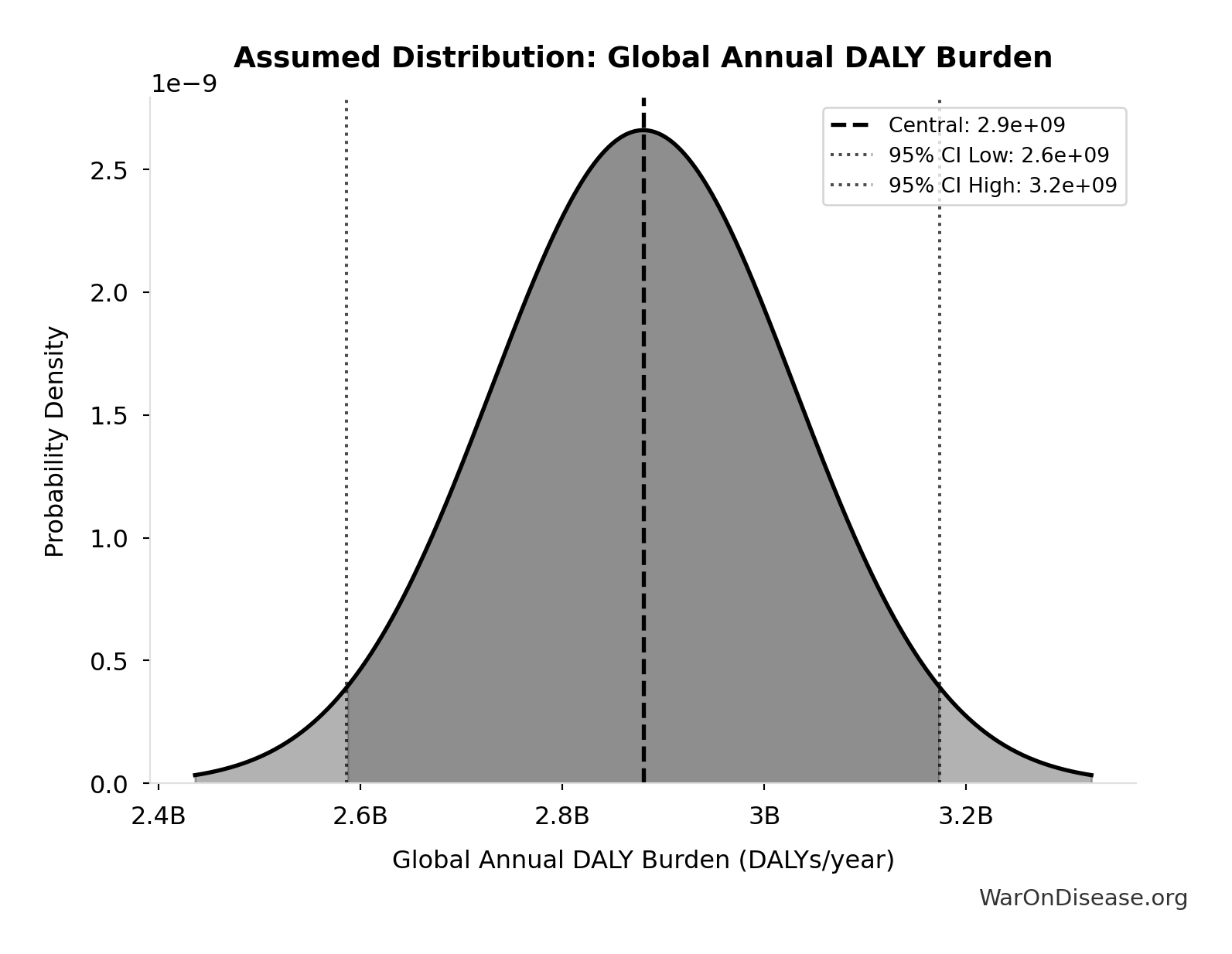
Global annual DALY burden from all diseases and injuries (WHO/IHME Global Burden of Disease 2021). Includes both YLL (years of life lost) and YLD (years lived with disability) from all causes.
Source:35
Uncertainty Range
Technical: Distribution: Normal (SE: 150 million DALYs/year)
Input Distribution
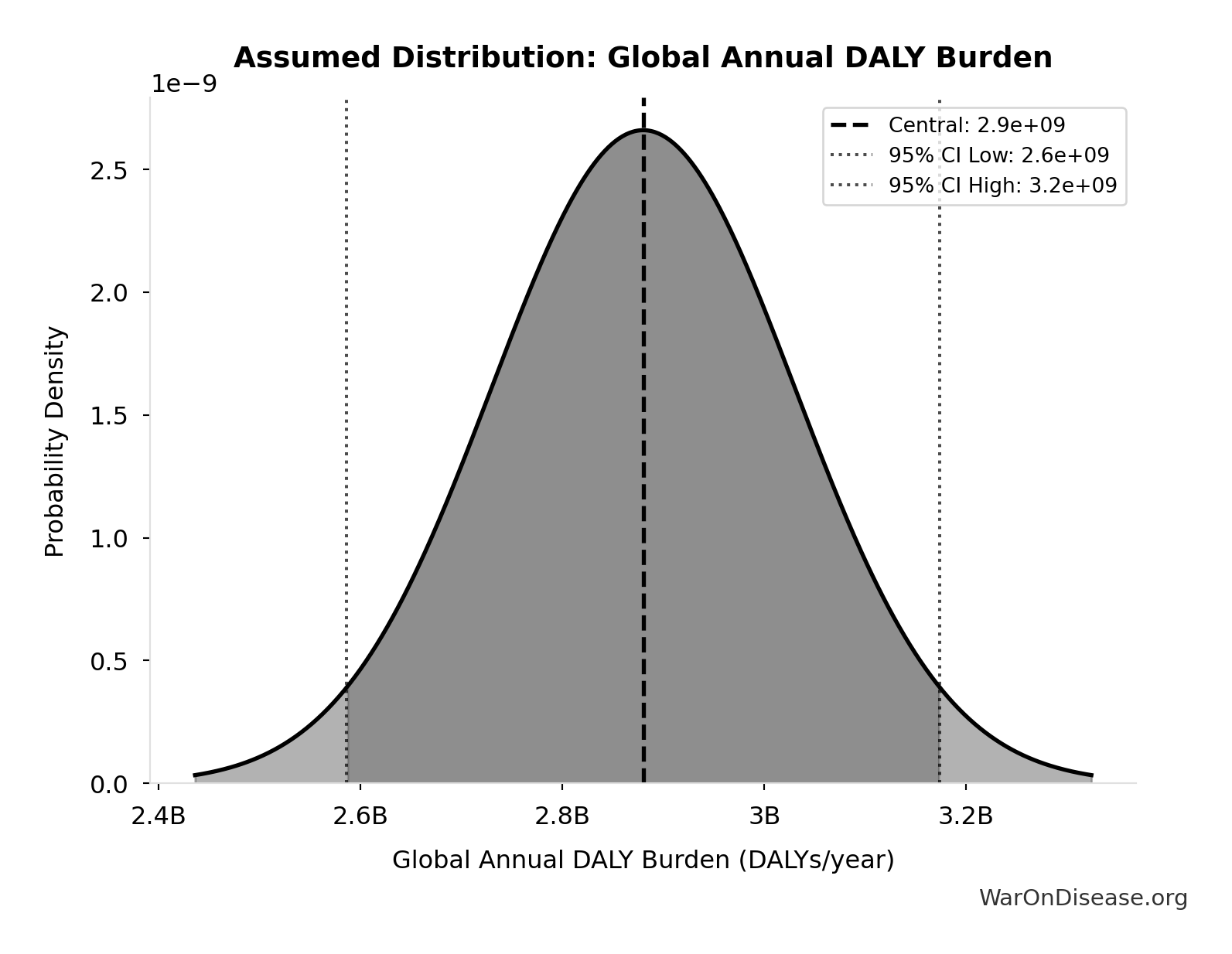
This chart shows the assumed probability distribution for this parameter. The shaded region represents the 95% confidence interval where we expect the true value to fall.
✓ High confidence • 📊 Peer-reviewed
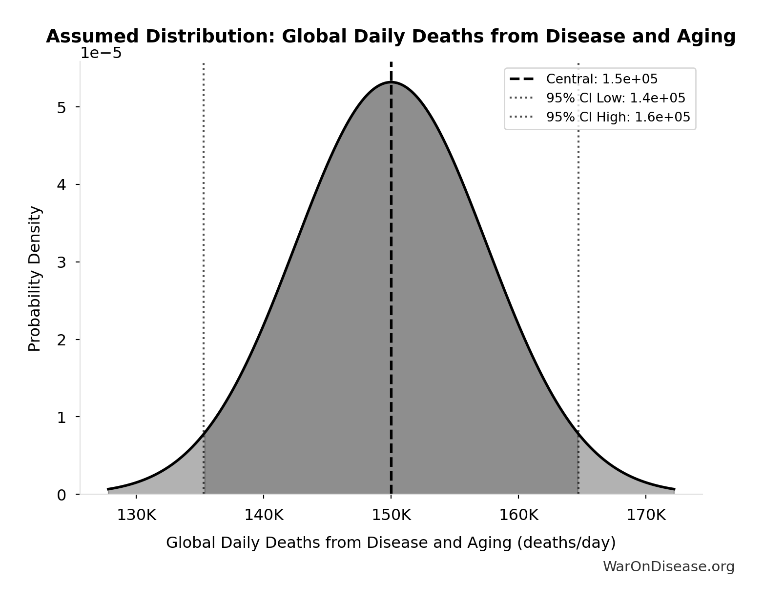
Global Daily Deaths from Disease and Aging: 150 thousand deaths/day
Note📊 Details
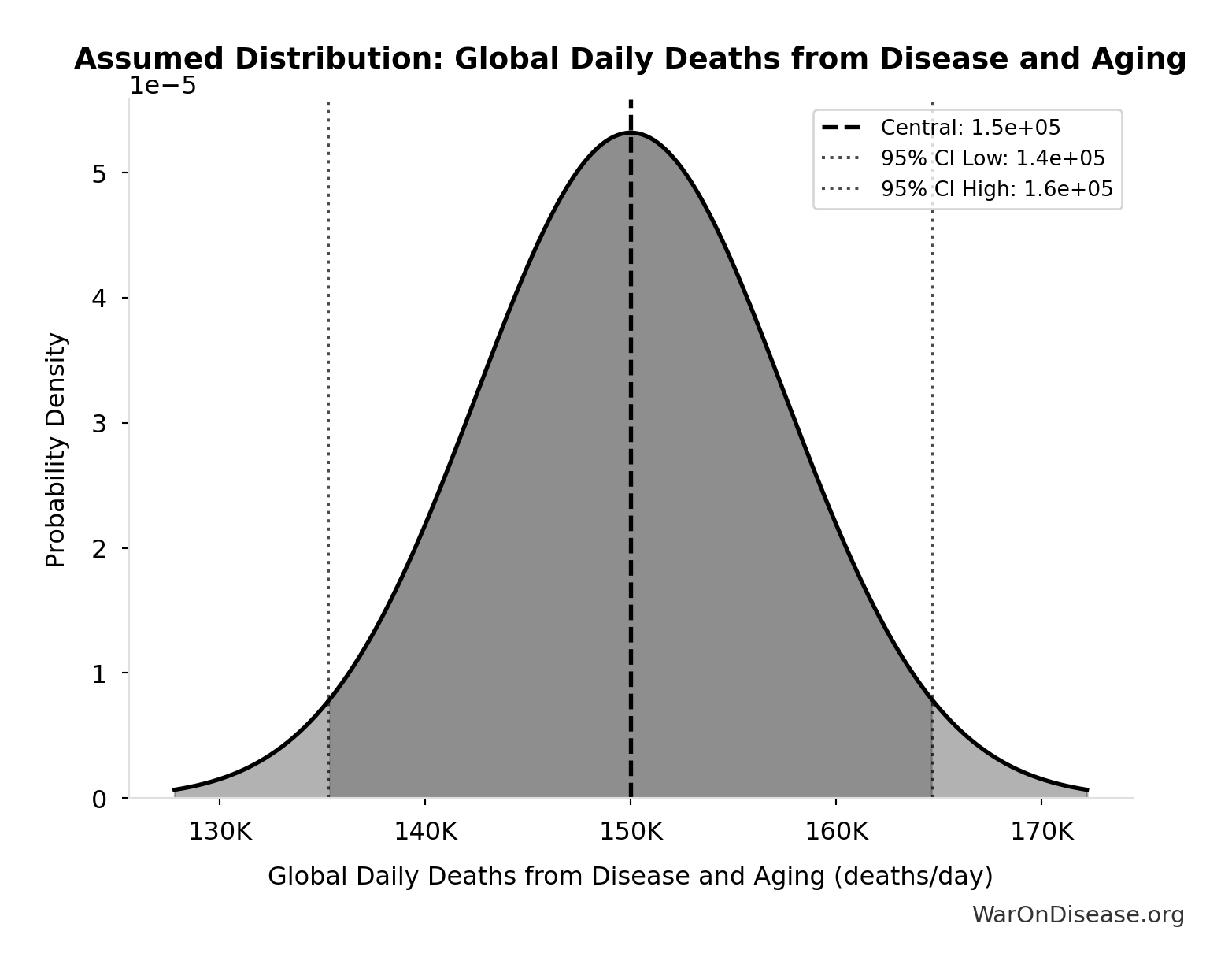
Total global deaths per day from all disease and aging (WHO Global Burden of Disease 2024)
Source:4
Uncertainty Range
Technical: Distribution: Normal (SE: 7.5 thousand deaths/day)
Input Distribution
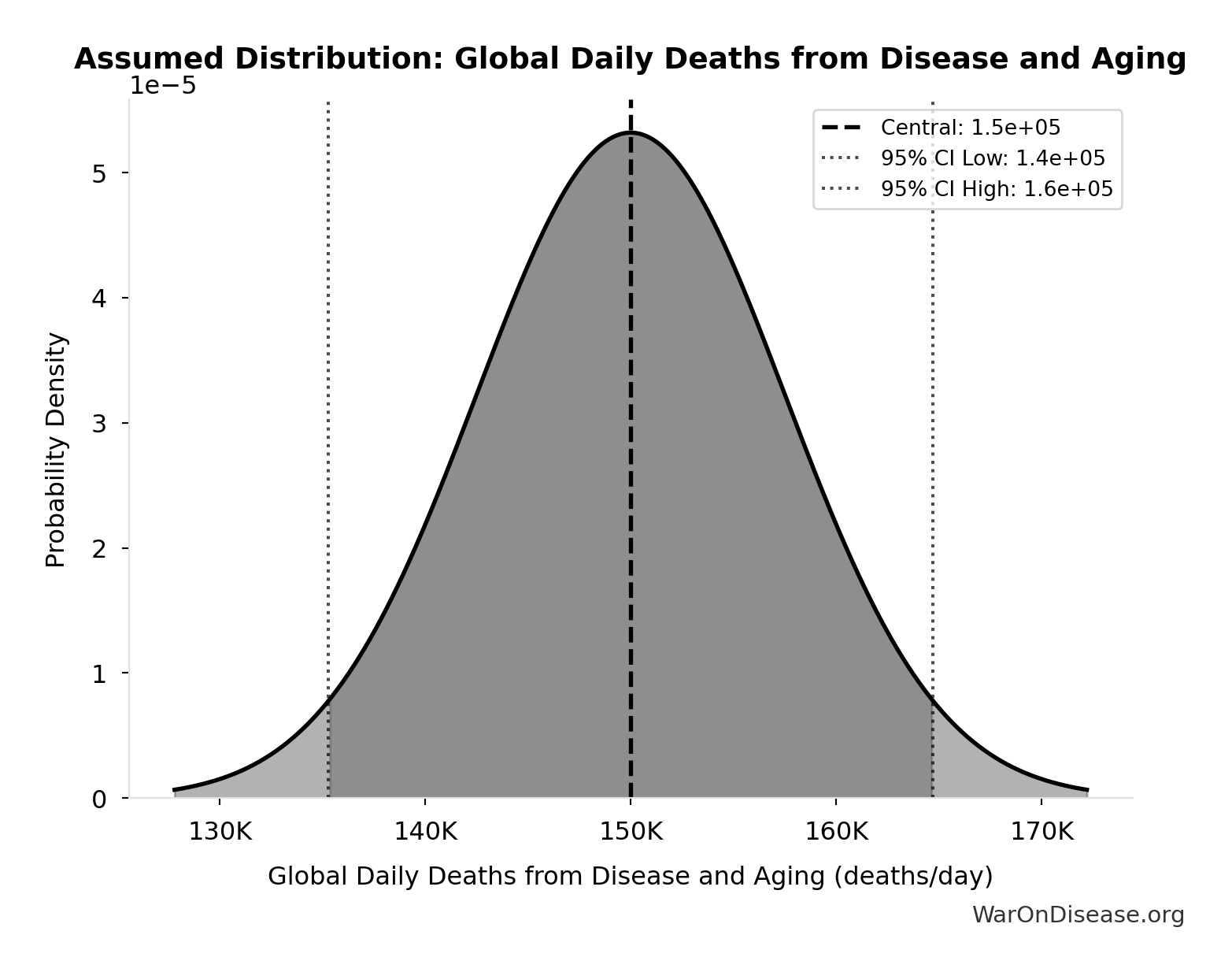
This chart shows the assumed probability distribution for this parameter. The shaded region represents the 95% confidence interval where we expect the true value to fall.
✓ High confidence • 📊 Peer-reviewed
Global GDP (2025): $115T
Note📊 Details
Global nominal GDP (2025 estimate). From Political Dysfunction Tax paper citing StatisticsTimes/IMF World Economic Outlook. Used for calculating global opportunity costs as percentage of world economic output. Note: Latest IMF data shows $117T.
Source:47
Uncertainty Range
Technical: Distribution: Fixed
✓ High confidence
Global Military Spending in 2024: $2.72T
Note📊 Details
Global military spending in 2024
Source:52
Uncertainty Range
Technical: Distribution: Fixed
✓ High confidence
Global Population 2045 (Projected): 9.2 billion of people
Note📊 Details
UN World Population Prospects 2022 median projection for 2045.
Source:56
Uncertainty Range
Technical: Distribution: Fixed
✓ High confidence
Diseases Getting First Treatment Per Year: 15 diseases/year
Note📊 Details
Number of diseases that receive their FIRST effective treatment each year under current system. ~9 rare diseases/year (based on 40 years of ODA: 350 with treatment ÷ 40 years), plus ~5-10 common diseases. Note: FDA approves ~50 drugs/year, but most are for diseases that already have treatments.
Source:68
Uncertainty Range
Technical: 95% CI: [8 diseases/year, 30 diseases/year] • Distribution: Lognormal
What this means: This estimate is highly uncertain. The true value likely falls between 8 diseases/year and 30 diseases/year (±73%). This represents a very wide range that our Monte Carlo simulations account for when calculating overall uncertainty in the results.
The lognormal distribution means values can’t go negative and have a longer tail toward higher values (common for costs and populations).
Input Distribution
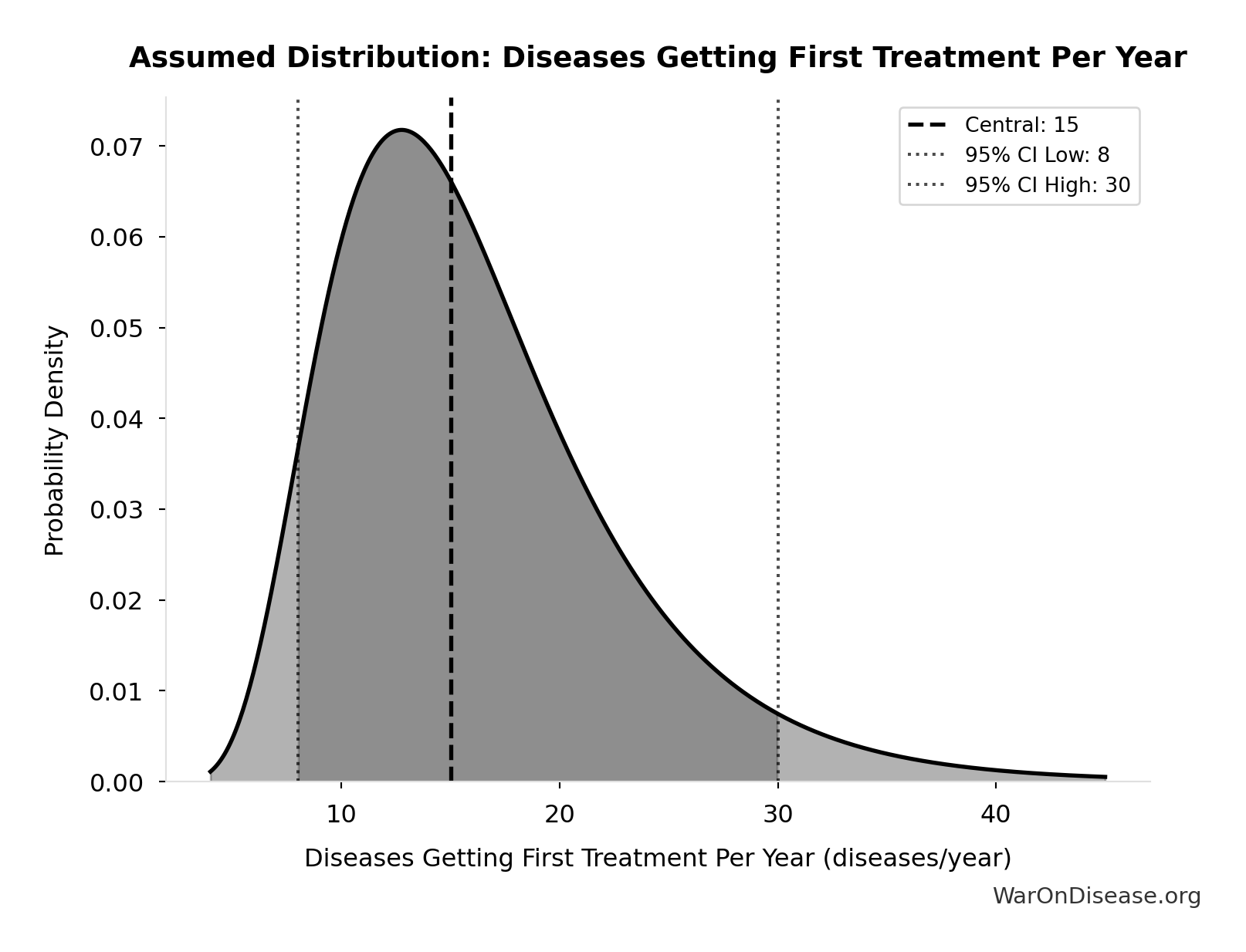
This chart shows the assumed probability distribution for this parameter. The shaded region represents the 95% confidence interval where we expect the true value to fall.
? Low confidence
Patient Willingness to Participate in Clinical Trials: 44.8%
Note📊 Details
Patient willingness to participate in drug trials (44.8% in surveys, 88% when actually approached)
Source:73
Uncertainty Range
Technical: 95% CI: [40%, 50%] • Distribution: Normal (SE: 2.5%)
What this means: This estimate has moderate uncertainty. The true value likely falls between 40% and 50% (±11%). This represents a reasonable range that our Monte Carlo simulations account for when calculating overall uncertainty in the results.
The normal distribution means values cluster around the center with equal chances of being higher or lower.
Input Distribution
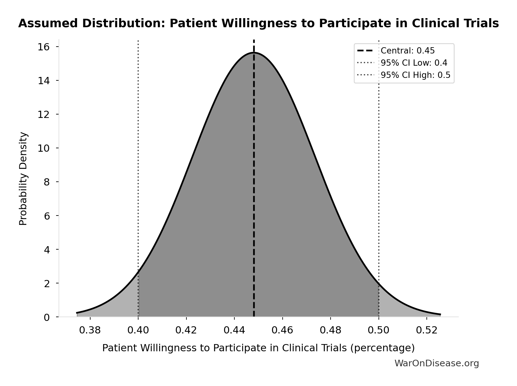
This chart shows the assumed probability distribution for this parameter. The shaded region represents the 95% confidence interval where we expect the true value to fall.
~ Medium confidence
Global Health Opportunity Cost: $34T
Note📊 Details
Annual opportunity cost of slow-motion regulatory environment for health innovation. Murphy-Topel (2006) valued cancer cure at $50T (inflation-adjusted ~$100T in 2025). Longevity dividend of 1 extra year = $38T globally. PCTs could accelerate cures by 10+ years; NPV of 10-year delay at 3% discount = ~$25T. Conservative estimate: $34T annually in lives lost and healthspan denied.
Source:47
Uncertainty Range
Technical: 95% CI: [$20T, $80T] • Distribution: Lognormal (SE: $15T)
What this means: This estimate is highly uncertain. The true value likely falls between $20T and $80T (±88%). This represents a very wide range that our Monte Carlo simulations account for when calculating overall uncertainty in the results.
The lognormal distribution means values can’t go negative and have a longer tail toward higher values (common for costs and populations).
Input Distribution
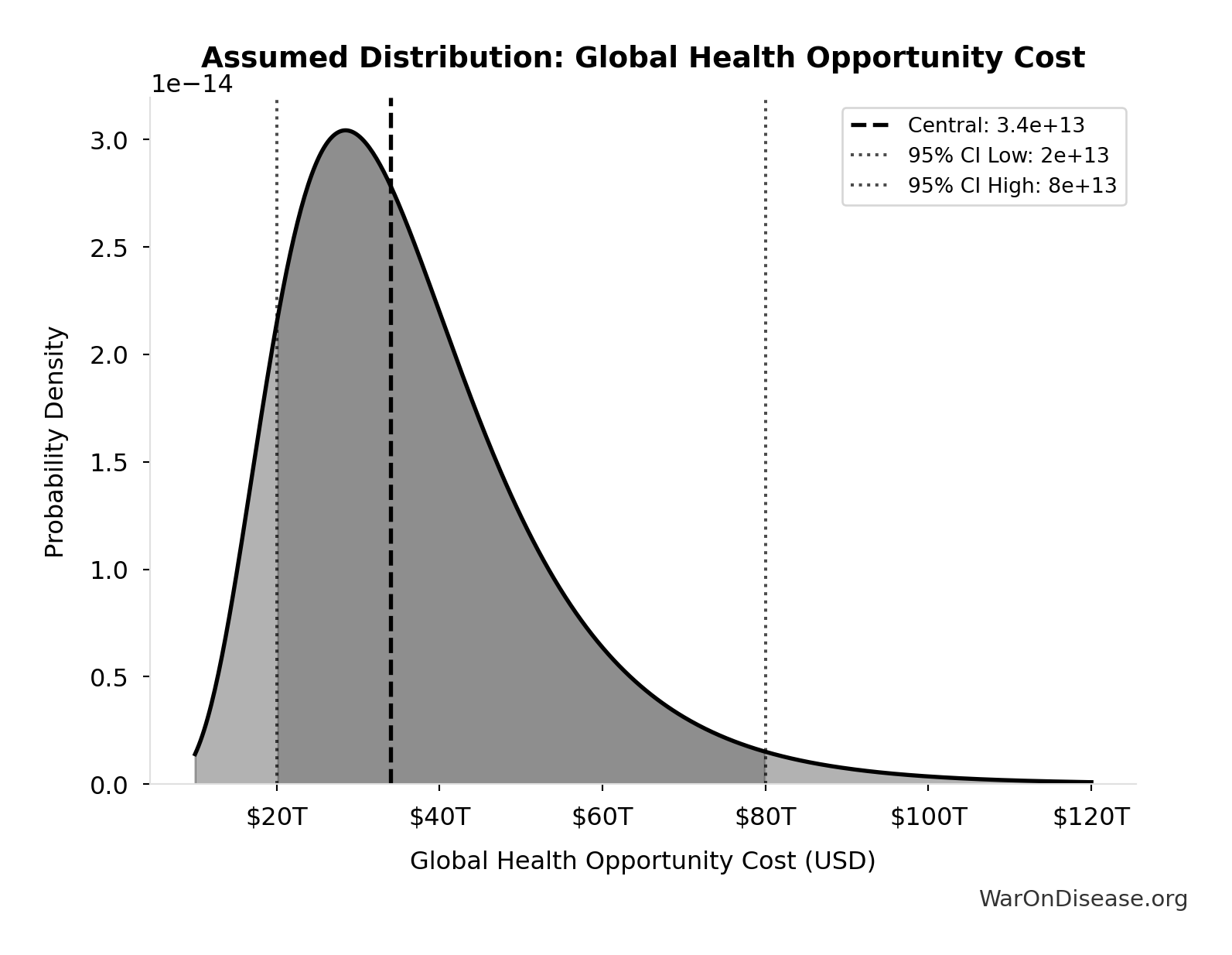
This chart shows the assumed probability distribution for this parameter. The shaded region represents the 95% confidence interval where we expect the true value to fall.
? Low confidence
Global Lead Poisoning Cost: $6T
Note📊 Details
Global cost of lead exposure: World Bank/Lancet estimate. 765 million IQ points lost annually, 5.5 million premature CVD deaths. Cost to eliminate lead from paint, spices, batteries is trivial compared to damage. This is an arbitrage opportunity of immense scale that governance has failed to execute.
Source:47
Uncertainty Range
Technical: 95% CI: [$4T, $8T] • Distribution: Normal (SE: $1T)
What this means: There’s significant uncertainty here. The true value likely falls between $4T and $8T (±33%). This represents a wide range that our Monte Carlo simulations account for when calculating overall uncertainty in the results.
The normal distribution means values cluster around the center with equal chances of being higher or lower.
Input Distribution
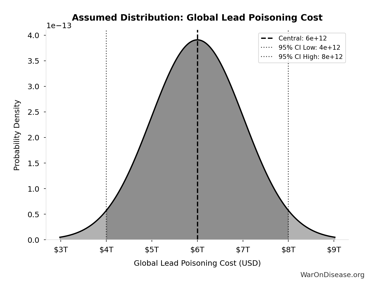
This chart shows the assumed probability distribution for this parameter. The shaded region represents the 95% confidence interval where we expect the true value to fall.
✓ High confidence
Global Migration Opportunity Cost: $57T
Note📊 Details
Unrealized output from migration restrictions. Clemens (2011) calculated eliminating labor mobility barriers could increase global GDP by 50-150%. At $115T global GDP, lower bound = $57T; upper bound = $170T. Even 5% workforce mobility would generate trillions, exceeding all foreign aid ever given. This is the largest single distortion in the global economy.
Source:47
Uncertainty Range
Technical: 95% CI: [$57T, $170T] • Distribution: Lognormal (SE: $30T)
What this means: This estimate is highly uncertain. The true value likely falls between $57T and $170T (±99%). This represents a very wide range that our Monte Carlo simulations account for when calculating overall uncertainty in the results.
The lognormal distribution means values can’t go negative and have a longer tail toward higher values (common for costs and populations).
Input Distribution
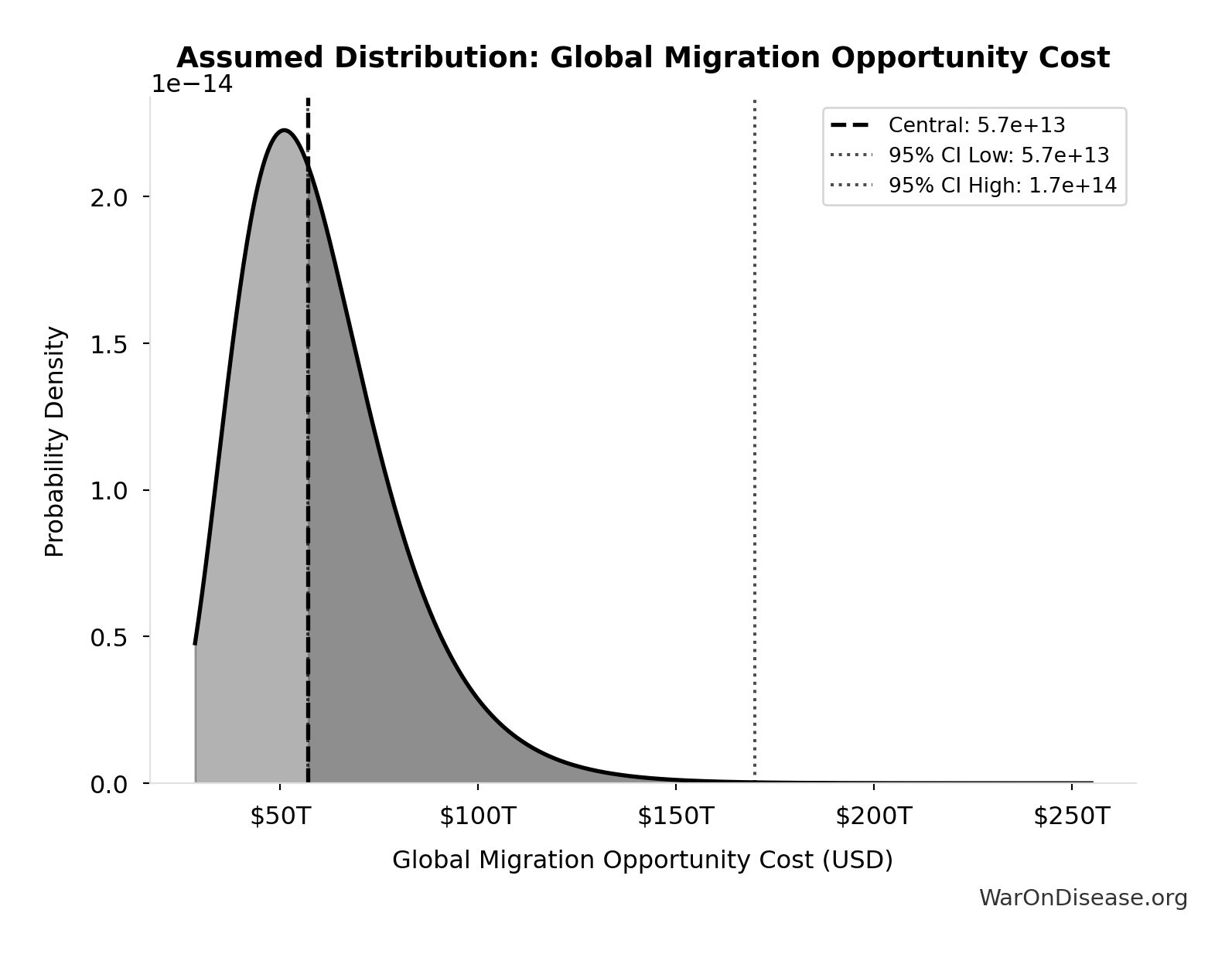
This chart shows the assumed probability distribution for this parameter. The shaded region represents the 95% confidence interval where we expect the true value to fall.
? Low confidence
Global Science Opportunity Cost: $4T
Note📊 Details
Annual opportunity cost from underfunding high-ROI science (fusion, AI safety). Human Genome Project: $3.8B cost, $796B-1T impact (141:1 ROI). Fusion DEMO plant: $5-10B could solve energy/climate permanently. AI safety: <5% of capabilities spending despite existential stakes. Reallocating $200B from military waste at 20x multiplier = $4T foregone growth.
Source:47
Uncertainty Range
Technical: 95% CI: [$2T, $10T] • Distribution: Lognormal (SE: $2T)
What this means: This estimate is highly uncertain. The true value likely falls between $2T and $10T (±100%). This represents a very wide range that our Monte Carlo simulations account for when calculating overall uncertainty in the results.
The lognormal distribution means values can’t go negative and have a longer tail toward higher values (common for costs and populations).
Input Distribution
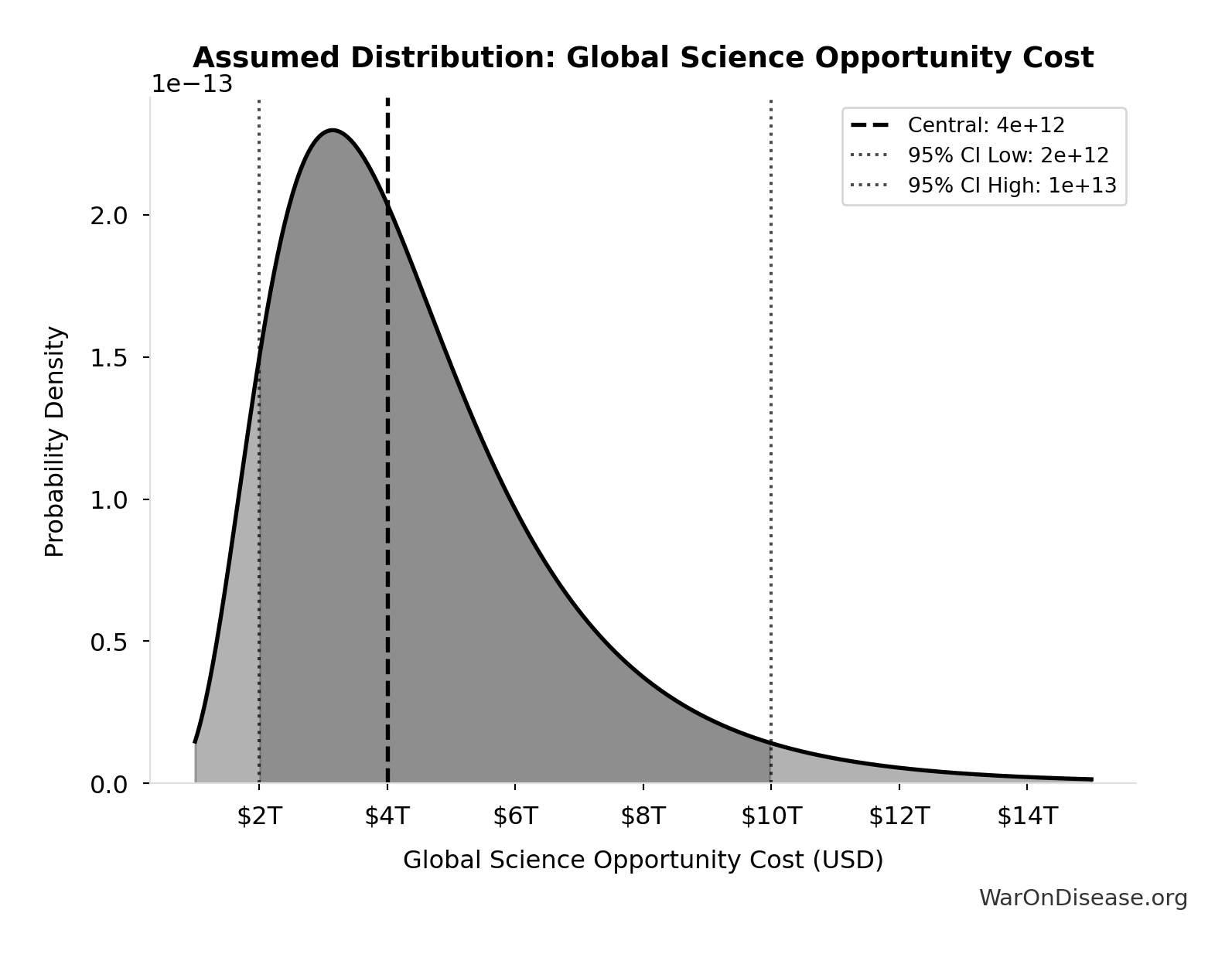
This chart shows the assumed probability distribution for this parameter. The shaded region represents the 95% confidence interval where we expect the true value to fall.
? Low confidence
Post-Office Career Value (per politician): $10M
Note📊 Details
Net present value of post-office career premium for average congressperson (10 years x $1M/year premium). Based on documented cases: Gephardt $7M/year, Daschle $2M+/year.
Source:83
Uncertainty Range
Technical: 95% CI: [$5M, $20M]
What this means: This estimate is highly uncertain. The true value likely falls between $5M and $20M (±75%). This represents a very wide range that our Monte Carlo simulations account for when calculating overall uncertainty in the results.
Input Distribution
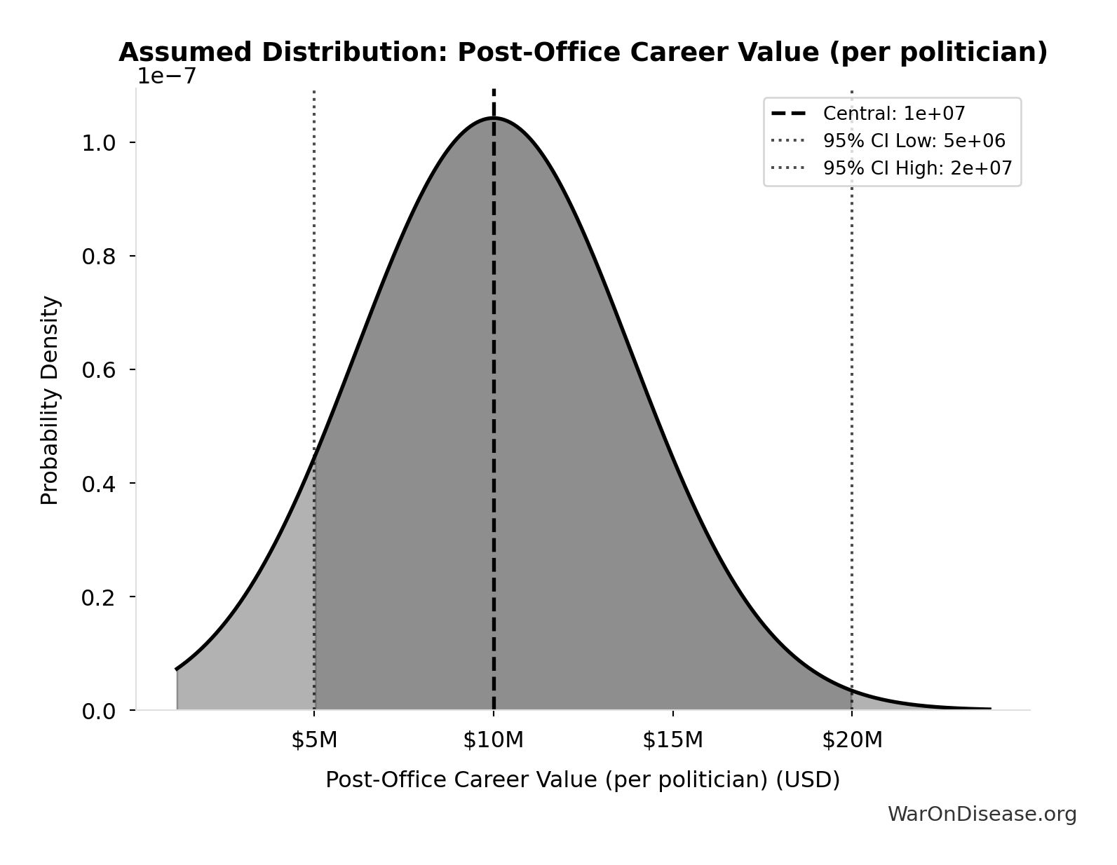
This chart shows the assumed probability distribution for this parameter. The shaded region represents the 95% confidence interval where we expect the true value to fall.
~ Medium confidence
Total Number of Rare Diseases Globally: 7 thousand diseases
Note📊 Details
Total number of rare diseases globally
Source:87
Uncertainty Range
Technical: 95% CI: [6 thousand diseases, 10 thousand diseases] • Distribution: Normal
What this means: There’s significant uncertainty here. The true value likely falls between 6 thousand diseases and 10 thousand diseases (±29%). This represents a wide range that our Monte Carlo simulations account for when calculating overall uncertainty in the results.
The normal distribution means values cluster around the center with equal chances of being higher or lower.
Input Distribution
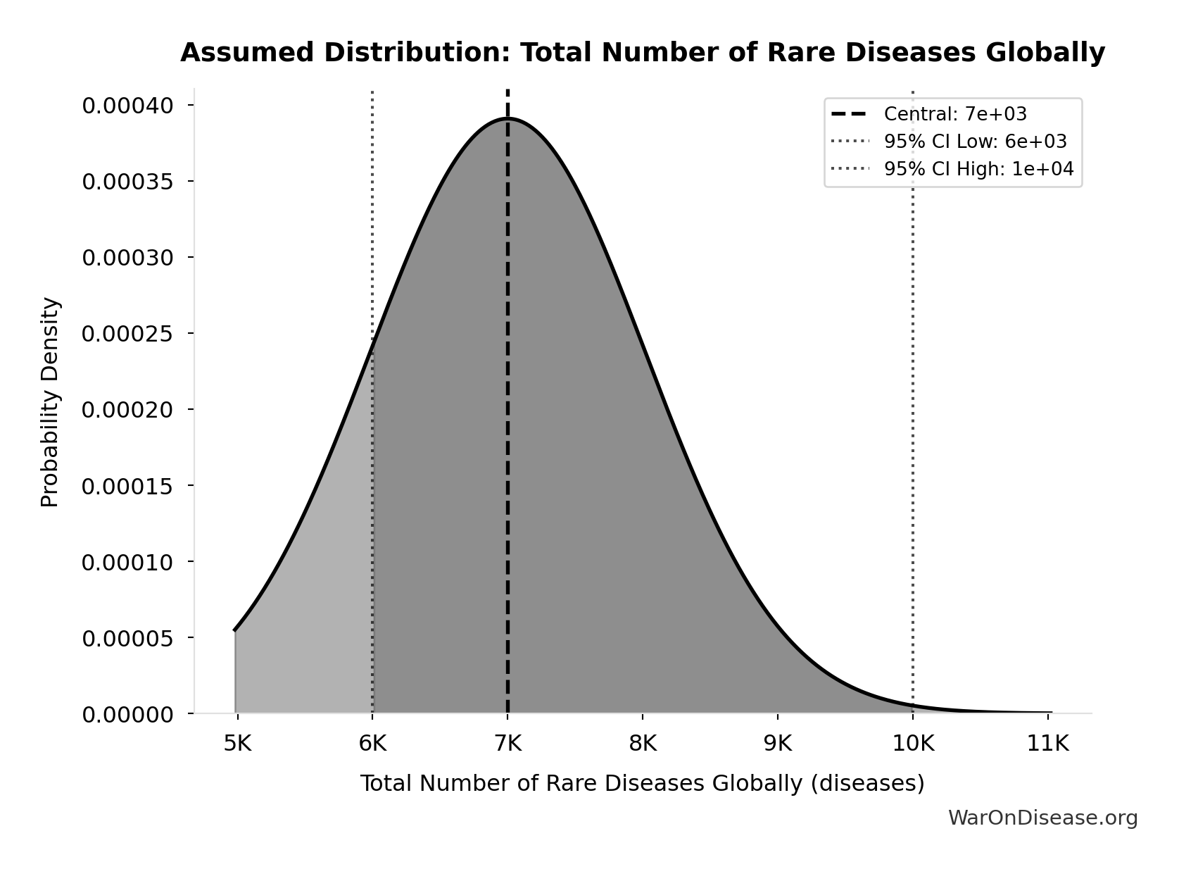
This chart shows the assumed probability distribution for this parameter. The shaded region represents the 95% confidence interval where we expect the true value to fall.
✓ High confidence
Standard Economic Value per QALY: $150K
Note📊 Details
Standard economic value per QALY
Source:96
Uncertainty Range
Technical: Distribution: Normal (SE: $30K)
Input Distribution
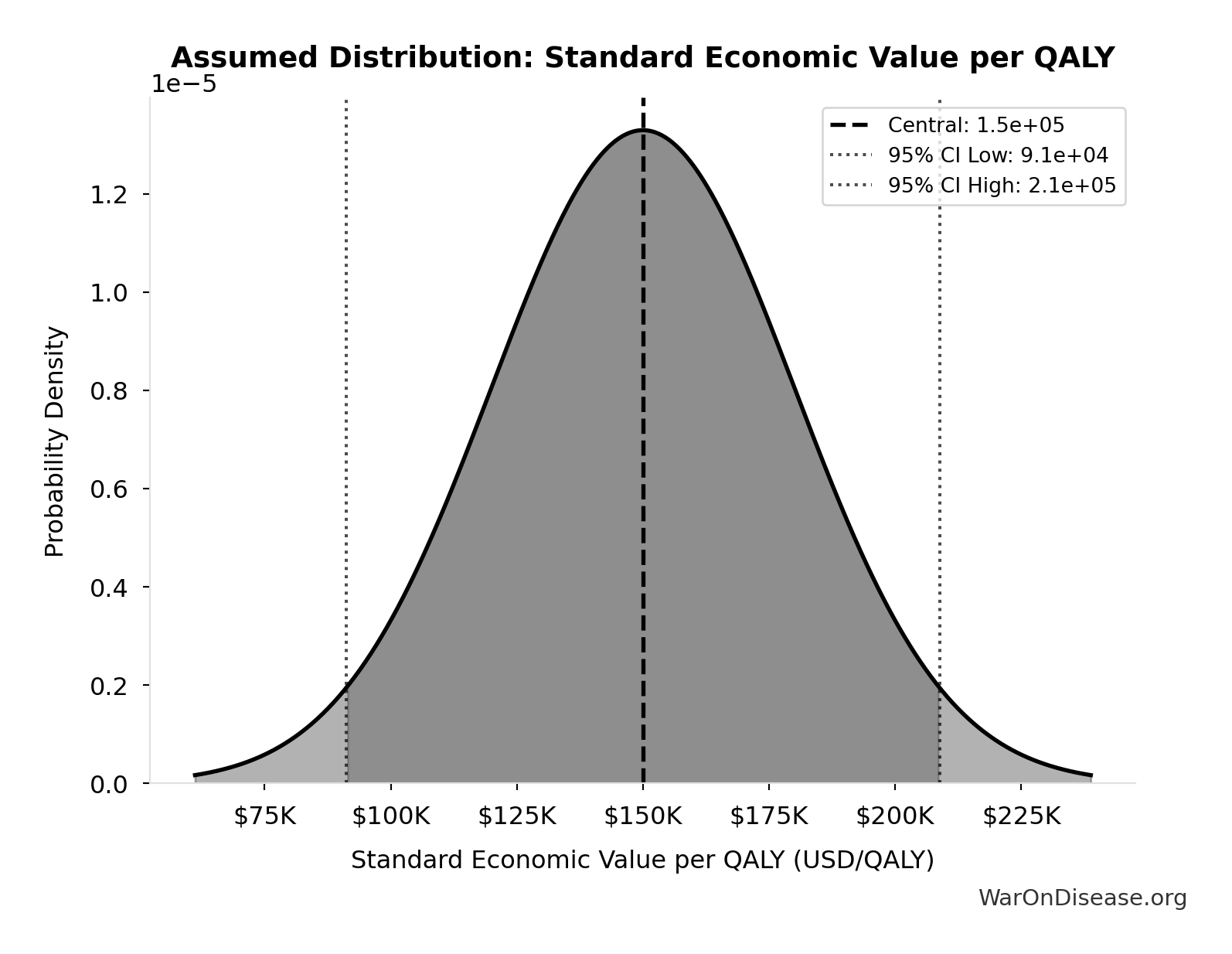
This chart shows the assumed probability distribution for this parameter. The shaded region represents the 95% confidence interval where we expect the true value to fall.
✓ High confidence
US Military Spending at WW2 Peak (Constant 2024 Dollars): $1.42T
Note📊 Details
US military spending at WW2 peak (1945) in constant 2024 dollars
Source:126
Uncertainty Range
Technical: Distribution: Fixed
✓ High confidence
US Military Spending in 1947 (Constant 2024 Dollars): $176B
Note📊 Details
US military spending in 1947 (post-WW2 trough, 2 years after peak) in constant 2024 dollars
Source:126
Uncertainty Range
Technical: Distribution: Fixed
✓ High confidence
Senators for Treaty Ratification: 67 senators
Note📊 Details
Senators needed for treaty ratification (2/3 majority per Article II, Section 2)
Source:129
Uncertainty Range
Technical: Distribution: Fixed
✓ High confidence
US Federal Campaign Spending (2024): $20B
Note📊 Details
Total US federal election spending in 2024 cycle including presidential, congressional, party committees, and PACs. Source: FEC Statistical Summary 2024.
Source:130
Uncertainty Range
Technical: 95% CI: [$18B, $22B]
What this means: We’re quite confident in this estimate. The true value likely falls between $18B and $22B (±10%). This represents a narrow range that our Monte Carlo simulations account for when calculating overall uncertainty in the results.
Input Distribution
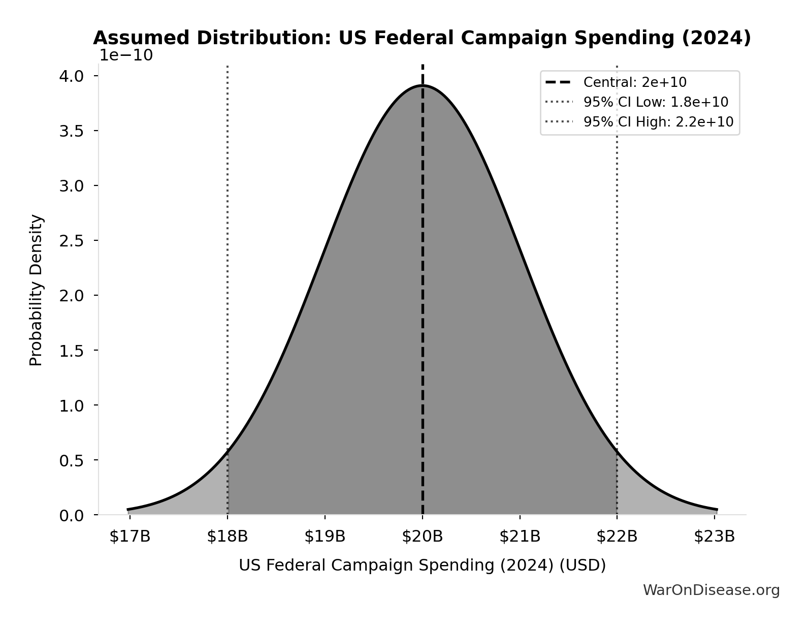
This chart shows the assumed probability distribution for this parameter. The shaded region represents the 95% confidence interval where we expect the true value to fall.
✓ High confidence
US Total Lobbying (2024): $4.4B
Note📊 Details
Total US federal lobbying expenditure in 2024 (record year). Source: OpenSecrets.
Source:131
Uncertainty Range
Technical: 95% CI: [$3.74B, $5.06B]
What this means: This estimate has moderate uncertainty. The true value likely falls between $3.74B and $5.06B (±15%). This represents a reasonable range that our Monte Carlo simulations account for when calculating overall uncertainty in the results.
Input Distribution
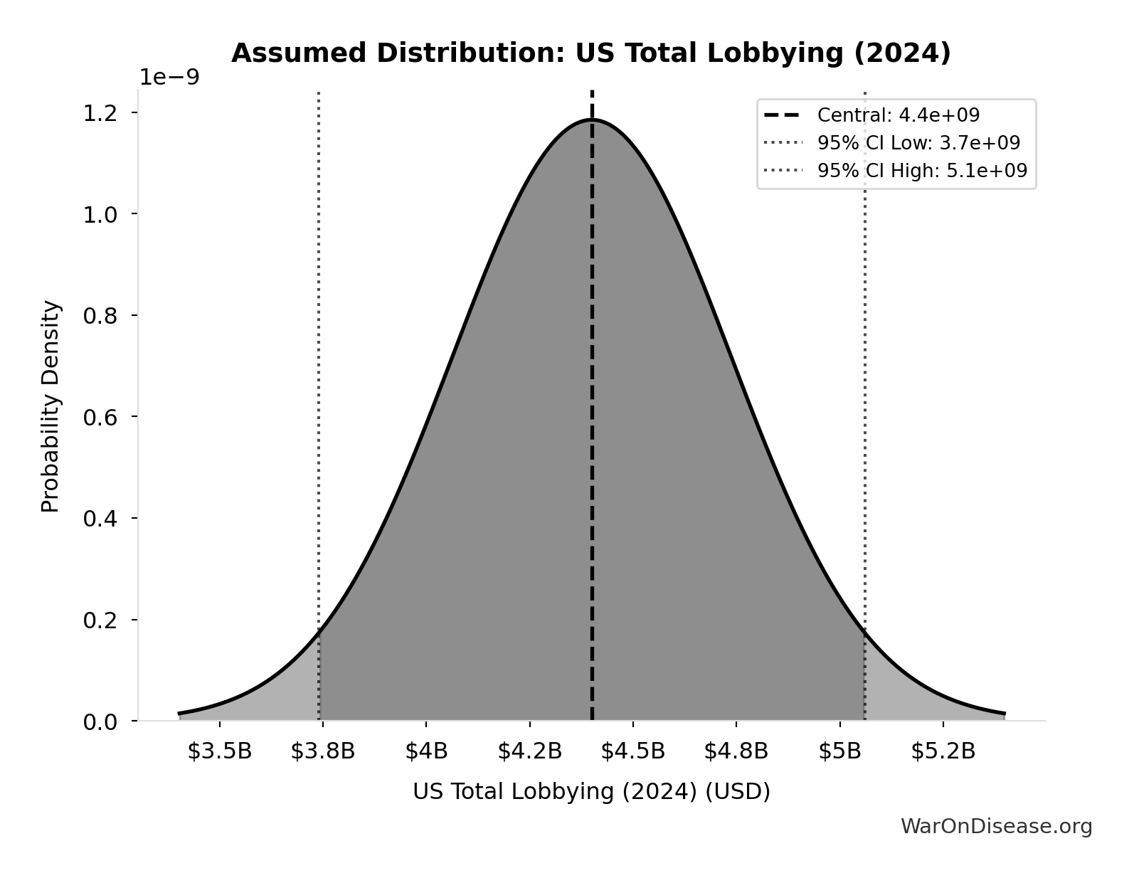
This chart shows the assumed probability distribution for this parameter. The shaded region represents the 95% confidence interval where we expect the true value to fall.
✓ High confidence
Core Definitions
Fundamental parameters and constants used throughout the analysis.
dFDA Annual Trial Funding: $21.8B
Note📊 Details
Assumed annual funding for dFDA pragmatic clinical trials (~$21.8B/year). Source-agnostic: could come from military reallocation, philanthropy, or government appropriation.
Uncertainty Range
Technical: Distribution: Fixed
Core definition
Decentralized Framework for Drug Assessment Community Support Costs: $2M
Note📊 Details
Decentralized Framework for Drug Assessment community support costs
Uncertainty Range
Technical: 95% CI: [$1M, $3M] • Distribution: Lognormal
What this means: There’s significant uncertainty here. The true value likely falls between $1M and $3M (±50%). This represents a wide range that our Monte Carlo simulations account for when calculating overall uncertainty in the results.
The lognormal distribution means values can’t go negative and have a longer tail toward higher values (common for costs and populations).
Input Distribution
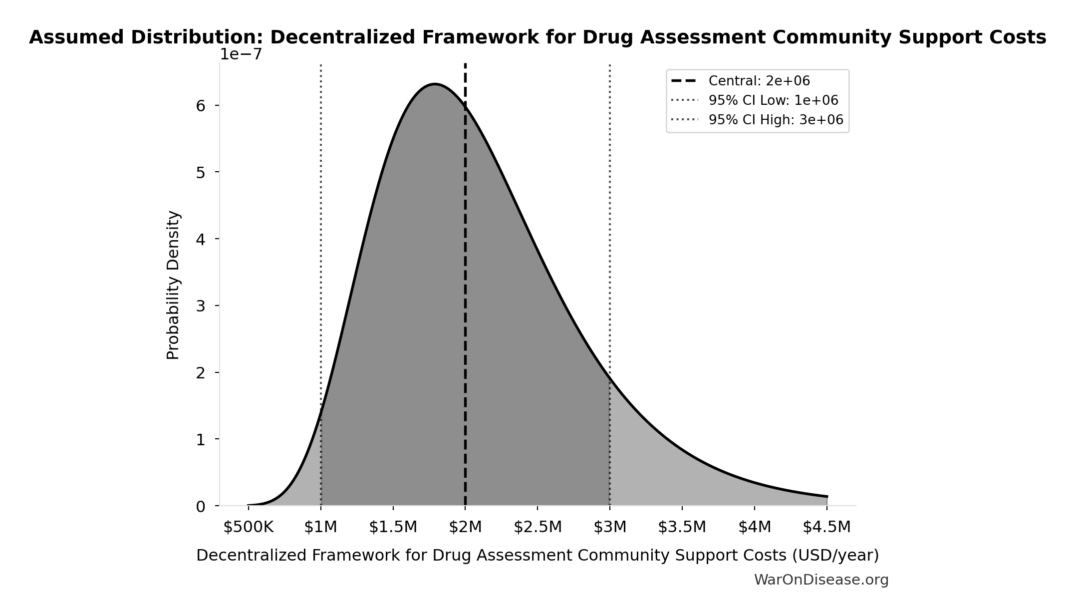
This chart shows the assumed probability distribution for this parameter. The shaded region represents the 95% confidence interval where we expect the true value to fall.
Core definition
Decentralized Framework for Drug Assessment Infrastructure Costs: $8M
Note📊 Details
Decentralized Framework for Drug Assessment infrastructure costs (cloud, security)
Uncertainty Range
Technical: 95% CI: [$5M, $12M] • Distribution: Lognormal
What this means: There’s significant uncertainty here. The true value likely falls between $5M and $12M (±44%). This represents a wide range that our Monte Carlo simulations account for when calculating overall uncertainty in the results.
The lognormal distribution means values can’t go negative and have a longer tail toward higher values (common for costs and populations).
Input Distribution
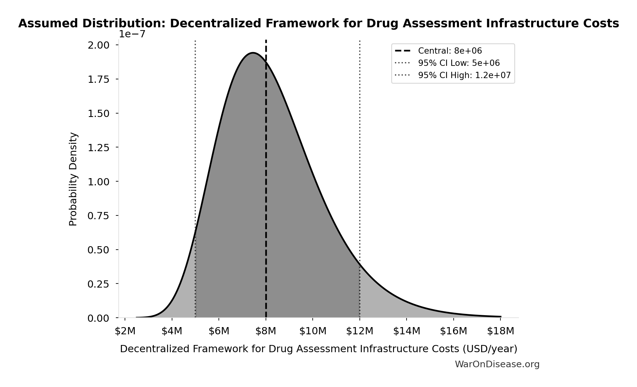
This chart shows the assumed probability distribution for this parameter. The shaded region represents the 95% confidence interval where we expect the true value to fall.
Core definition
Decentralized Framework for Drug Assessment Maintenance Costs: $15M
Note📊 Details
Decentralized Framework for Drug Assessment maintenance costs
Uncertainty Range
Technical: 95% CI: [$10M, $22M] • Distribution: Lognormal
What this means: There’s significant uncertainty here. The true value likely falls between $10M and $22M (±40%). This represents a wide range that our Monte Carlo simulations account for when calculating overall uncertainty in the results.
The lognormal distribution means values can’t go negative and have a longer tail toward higher values (common for costs and populations).
Input Distribution
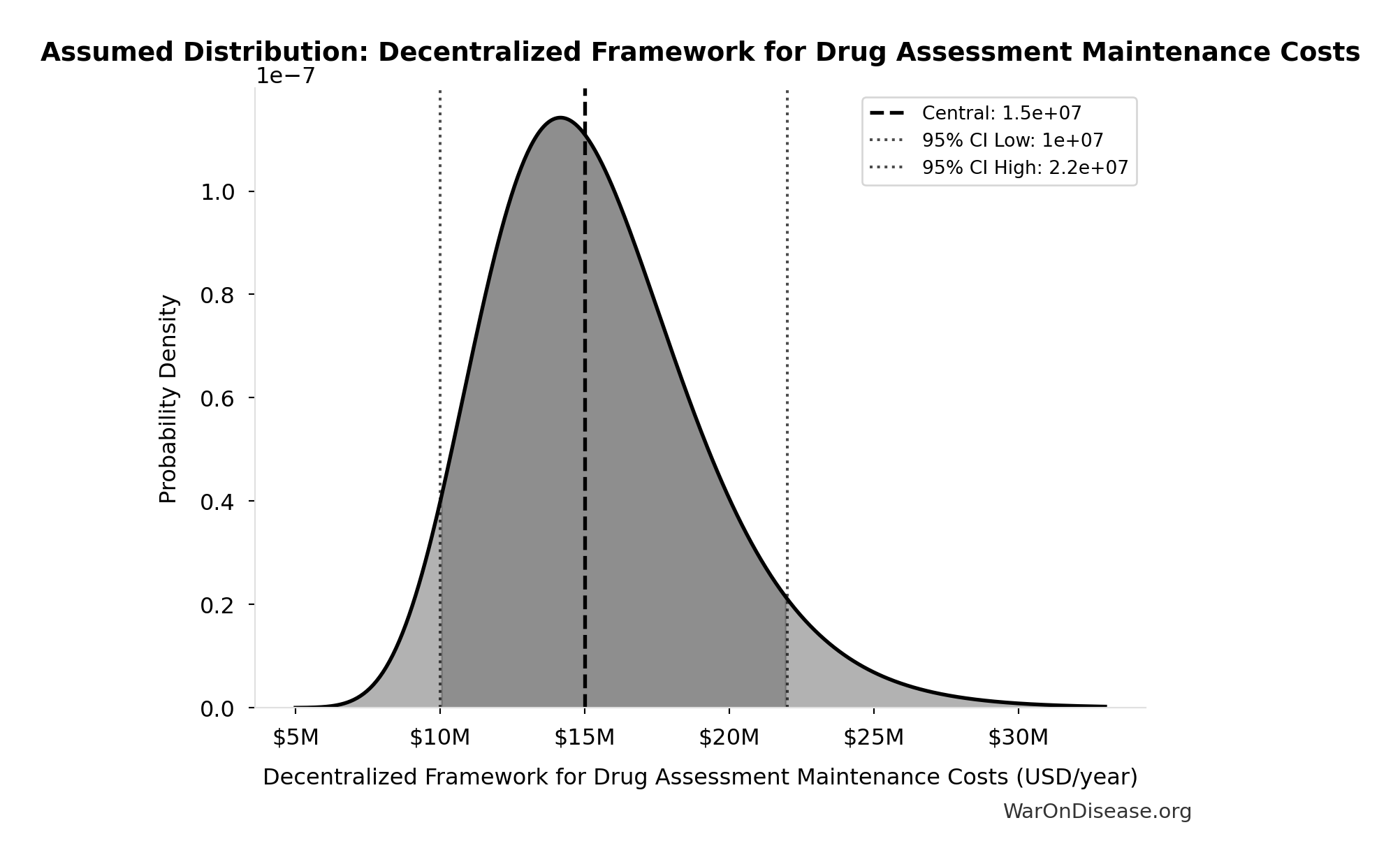
This chart shows the assumed probability distribution for this parameter. The shaded region represents the 95% confidence interval where we expect the true value to fall.
Core definition
Decentralized Framework for Drug Assessment Regulatory Coordination Costs: $5M
Note📊 Details
Decentralized Framework for Drug Assessment regulatory coordination costs
Uncertainty Range
Technical: 95% CI: [$3M, $8M] • Distribution: Lognormal
What this means: There’s significant uncertainty here. The true value likely falls between $3M and $8M (±50%). This represents a wide range that our Monte Carlo simulations account for when calculating overall uncertainty in the results.
The lognormal distribution means values can’t go negative and have a longer tail toward higher values (common for costs and populations).
Input Distribution
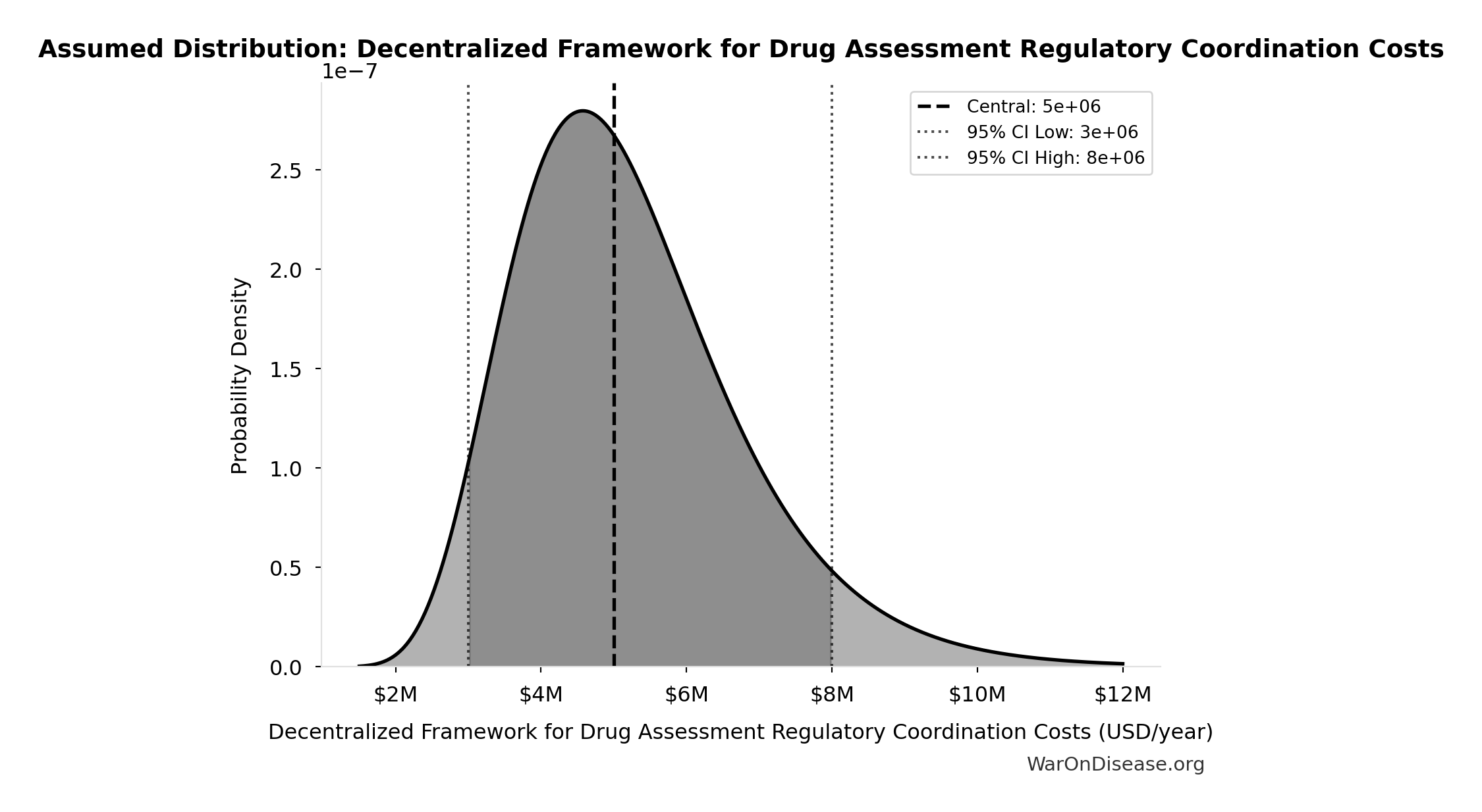
This chart shows the assumed probability distribution for this parameter. The shaded region represents the 95% confidence interval where we expect the true value to fall.
Core definition
Decentralized Framework for Drug Assessment Staff Costs: $10M
Note📊 Details
Decentralized Framework for Drug Assessment staff costs (minimal, AI-assisted)
Uncertainty Range
Technical: 95% CI: [$7M, $15M] • Distribution: Lognormal
What this means: There’s significant uncertainty here. The true value likely falls between $7M and $15M (±40%). This represents a wide range that our Monte Carlo simulations account for when calculating overall uncertainty in the results.
The lognormal distribution means values can’t go negative and have a longer tail toward higher values (common for costs and populations).
Input Distribution
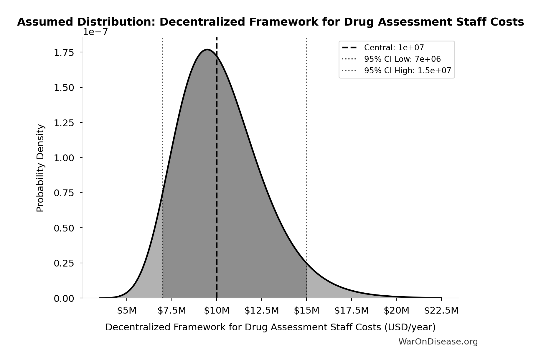
This chart shows the assumed probability distribution for this parameter. The shaded region represents the 95% confidence interval where we expect the true value to fall.
Core definition
Eventually Avoidable DALY Percentage: 92.6%
Note📊 Details
Percentage of DALYs that are eventually avoidable with sufficient biomedical research. Uses same methodology as EVENTUALLY_AVOIDABLE_DEATH_PCT. Most non-fatal chronic conditions (arthritis, depression, chronic pain) are also addressable through research, so the percentage is similar to deaths.
Uncertainty Range
Technical: 95% CI: [50%, 98%] • Distribution: Beta
What this means: There’s significant uncertainty here. The true value likely falls between 50% and 98% (±26%). This represents a wide range that our Monte Carlo simulations account for when calculating overall uncertainty in the results.
The beta distribution means values are bounded and can skew toward one end.
Input Distribution
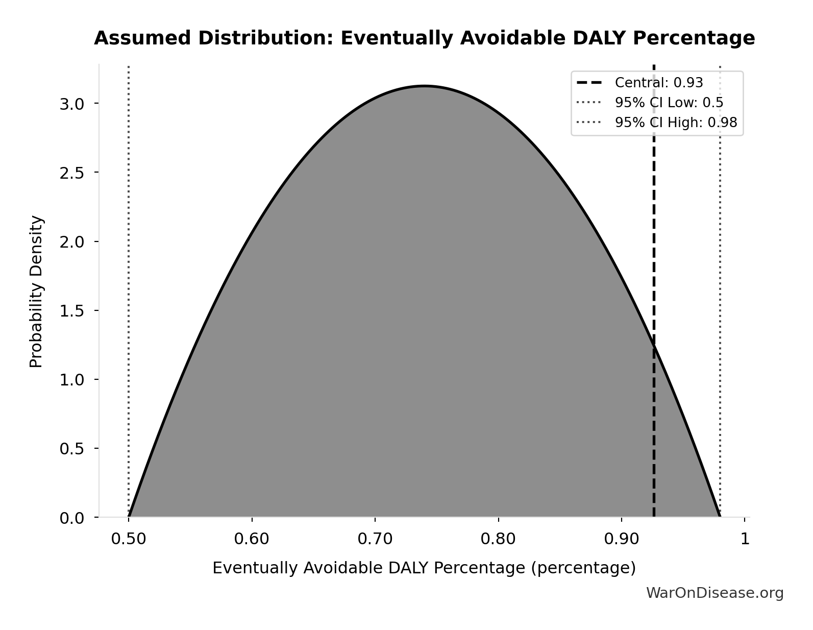
This chart shows the assumed probability distribution for this parameter. The shaded region represents the 95% confidence interval where we expect the true value to fall.
Core definition
Baseline Global GDP Growth Rate: 2.5%
Note📊 Details
Status-quo baseline annual global GDP growth rate.
Uncertainty Range
Technical: Distribution: Fixed
Core definition
Global-to-US Political Cost Ratio: 5:1
Note📊 Details
Ratio of global to US political reform costs. Based on discretionary spending ratio (~9x) discounted by ~50% for less transparent/expensive non-US political systems. Range 3-8 reflects uncertainty about non-US political dynamics and hidden influence channels.
Uncertainty Range
Technical: 95% CI: [3:1, 8:1] • Distribution: Lognormal
What this means: There’s significant uncertainty here. The true value likely falls between 3:1 and 8:1 (±50%). This represents a wide range that our Monte Carlo simulations account for when calculating overall uncertainty in the results.
The lognormal distribution means values can’t go negative and have a longer tail toward higher values (common for costs and populations).
Input Distribution
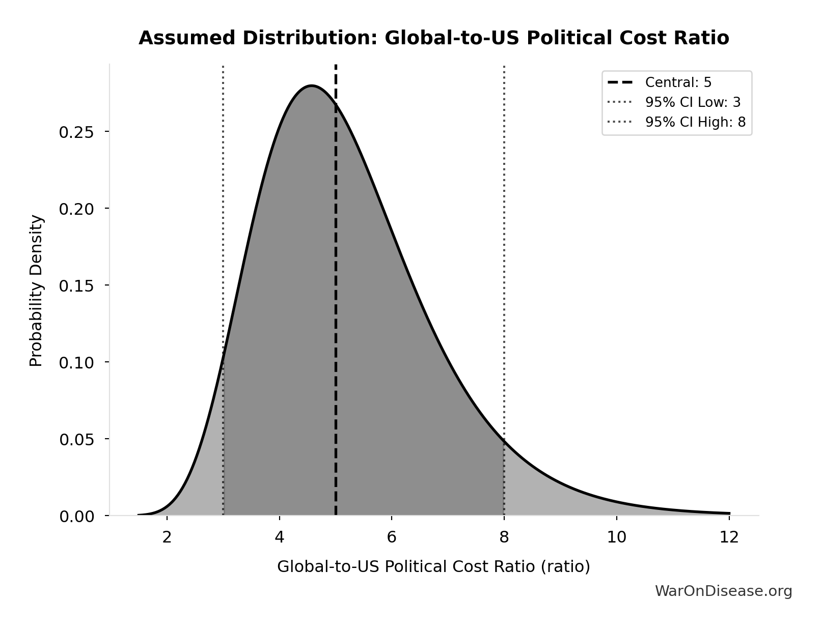
This chart shows the assumed probability distribution for this parameter. The shaded region represents the 95% confidence interval where we expect the true value to fall.
Core definition
GDP Growth Boost at 30% Military Reallocation: 5.5%
Note📊 Details
Historical calibration target: 30% military reallocation maps to ~5.5 percentage points annual GDP growth boost.
Uncertainty Range
Technical: 95% CI: [3.5%, 7.5%] • Distribution: Normal (SE: 1%)
What this means: There’s significant uncertainty here. The true value likely falls between 3.5% and 7.5% (±36%). This represents a wide range that our Monte Carlo simulations account for when calculating overall uncertainty in the results.
The normal distribution means values cluster around the center with equal chances of being higher or lower.
Input Distribution
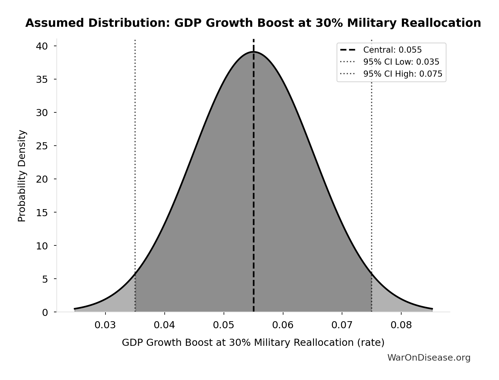
This chart shows the assumed probability distribution for this parameter. The shaded region represents the 95% confidence interval where we expect the true value to fall.
Core definition
R&D Spillover Multiplier: 2x
Note📊 Details
R&D spillover multiplier: each $1 in directed medical research produces $2 in adjacent sector GDP growth (biotech, AI, computing, materials science, manufacturing). Conservative estimate; military R&D spillover produced the internet, GPS, jet engines. Medical R&D spillover already produced CRISPR, mRNA platforms, AI protein folding.
Uncertainty Range
Technical: 95% CI: [1.5x, 2.5x] • Distribution: Normal (SE: 0.25x)
What this means: This estimate has moderate uncertainty. The true value likely falls between 1.5x and 2.5x (±25%). This represents a reasonable range that our Monte Carlo simulations account for when calculating overall uncertainty in the results.
The normal distribution means values cluster around the center with equal chances of being higher or lower.
Input Distribution
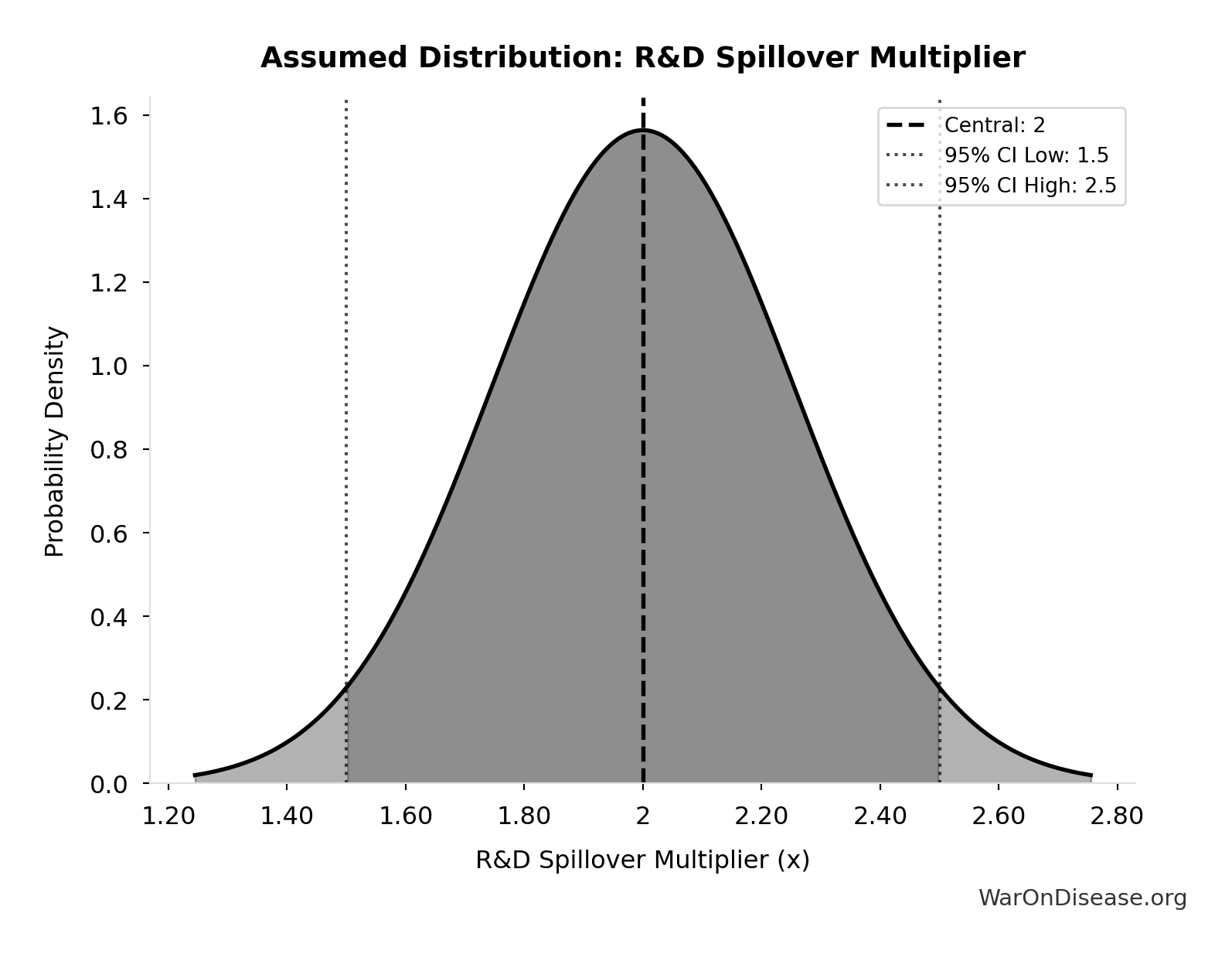
This chart shows the assumed probability distribution for this parameter. The shaded region represents the 95% confidence interval where we expect the true value to fall.
Core definition
Political Lobbying Campaign: Direct Lobbying, Super Pacs, Opposition Research, Staff, Legal/Compliance: $650M
Note📊 Details
Political lobbying campaign: direct lobbying (US/EU/G20), Super PACs, opposition research, staff, legal/compliance. Budget exceeds combined pharma ($300M/year) and military-industrial complex ($150M/year) lobbying to ensure competitive positioning. Referendum relies on grassroots mobilization and earned media, while lobbying requires matching or exceeding opposition spending for political viability.
Uncertainty Range
Technical: 95% CI: [$325M, $1.3B] • Distribution: Lognormal
What this means: This estimate is highly uncertain. The true value likely falls between $325M and $1.3B (±75%). This represents a very wide range that our Monte Carlo simulations account for when calculating overall uncertainty in the results.
The lognormal distribution means values can’t go negative and have a longer tail toward higher values (common for costs and populations).
Input Distribution
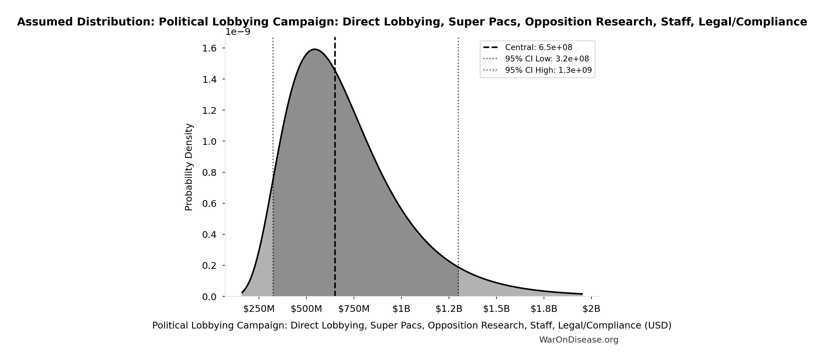
This chart shows the assumed probability distribution for this parameter. The shaded region represents the 95% confidence interval where we expect the true value to fall.
Core definition
Reserve Fund / Contingency Buffer: $100M
Note📊 Details
Reserve fund / contingency buffer (10% of total campaign cost). Using industry standard 10% for complex campaigns with potential for unforeseen legal challenges, opposition response, or regulatory delays. Conservative lower bound of $20M (2%) reflects transparent budget allocation and predictable referendum/lobbying costs.
Uncertainty Range
Technical: 95% CI: [$20M, $150M] • Distribution: Lognormal
What this means: This estimate is highly uncertain. The true value likely falls between $20M and $150M (±65%). This represents a very wide range that our Monte Carlo simulations account for when calculating overall uncertainty in the results.
The lognormal distribution means values can’t go negative and have a longer tail toward higher values (common for costs and populations).
Input Distribution
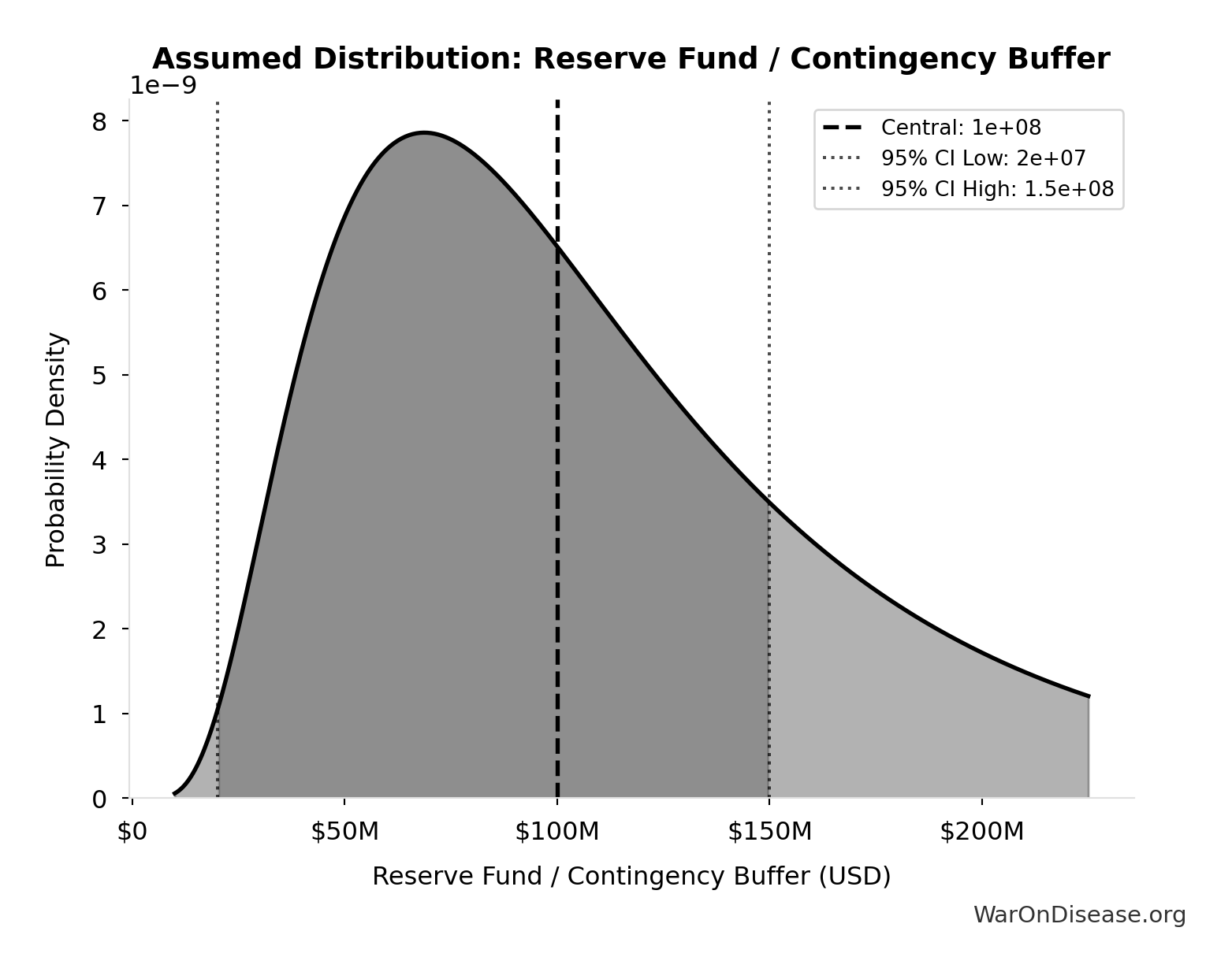
This chart shows the assumed probability distribution for this parameter. The shaded region represents the 95% confidence interval where we expect the true value to fall.
Core definition
Viral Referendum Budget: $250M
Note📊 Details
Viral referendum budget for 280M verified votes (base: $250M realistic with $0.50/vote avg, range: $150M optimistic $0.20/vote to $410M worst-case $1.05/vote). Components: platform ($35M), verification infrastructure (280M × friction × $0.18-0.20), tiered referral payments (varies by virality and marginal cost curve per diffusion theory), marketing seed ($5-15M). Based on PayPal referral economics ($18-36 inflation-adjusted) and biometric verification pricing ($0.15-0.25 at 300M+ scale).
Uncertainty Range
Technical: 95% CI: [$150M, $410M]
What this means: This estimate is highly uncertain. The true value likely falls between $150M and $410M (±52%). This represents a very wide range that our Monte Carlo simulations account for when calculating overall uncertainty in the results.
Input Distribution
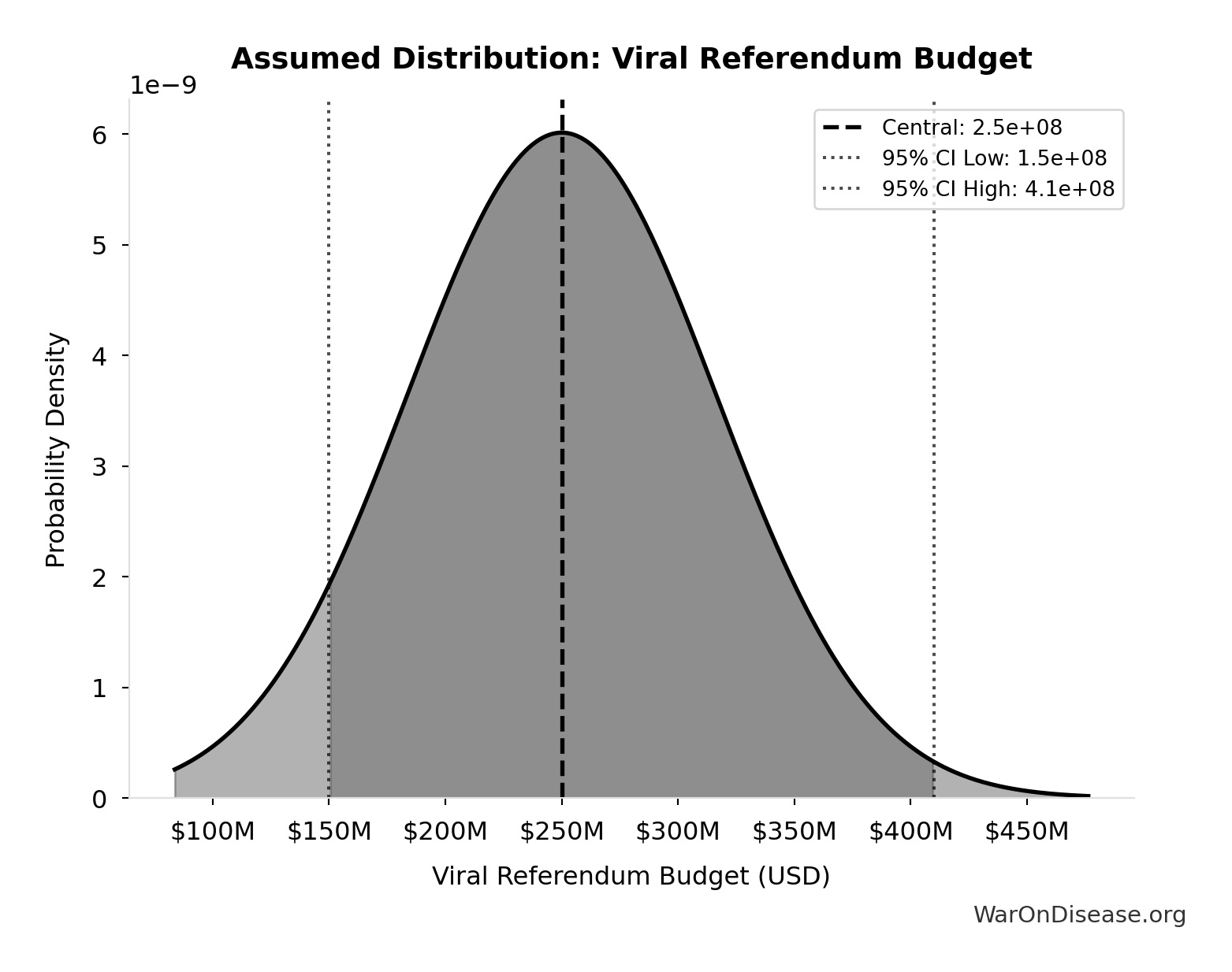
This chart shows the assumed probability distribution for this parameter. The shaded region represents the 95% confidence interval where we expect the true value to fall.
Core definition
1% Reduction in Military Spending/War Costs from Treaty: 1%
Note📊 Details
1% reduction in military spending/war costs from treaty
Uncertainty Range
Technical: Distribution: Fixed
Core definition
US Congress Members: 535 members
Note📊 Details
Total members of US Congress (100 senators + 435 representatives)
Uncertainty Range
Technical: Distribution: Fixed
Core definition
Political Effort Multiplier (US): 0.7x
Note📊 Details
Fraction of campaign + lobbying spending needed to achieve policy reform. Accounts for efficiency gains from coordination, message clarity, and public interest alignment. Range 0.4-1.2 reflects uncertainty about political dynamics.
Uncertainty Range
Technical: 95% CI: [0.4x, 1.2x] • Distribution: Lognormal
What this means: This estimate is highly uncertain. The true value likely falls between 0.4x and 1.2x (±57%). This represents a very wide range that our Monte Carlo simulations account for when calculating overall uncertainty in the results.
The lognormal distribution means values can’t go negative and have a longer tail toward higher values (common for costs and populations).
Input Distribution
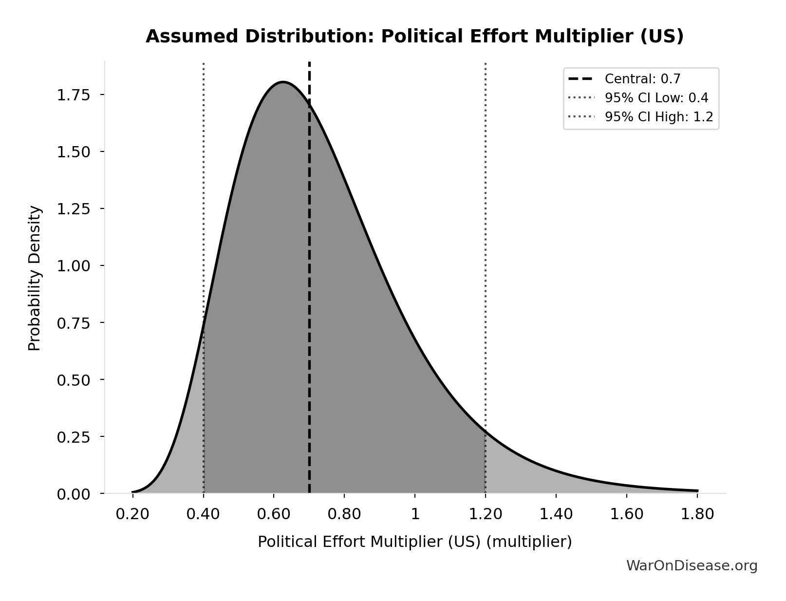
This chart shows the assumed probability distribution for this parameter. The shaded region represents the 95% confidence interval where we expect the true value to fall.
Core definition
References
1.
NIH Common Fund. NIH pragmatic trials: Minimal funding despite 30x cost advantage. NIH Common Fund: HCS Research Collaboratory https://commonfund.nih.gov/hcscollaboratory (2025)
The NIH Pragmatic Trials Collaboratory funds trials at $500K for planning phase, $1M/year for implementation-a tiny fraction of NIH’s budget. The ADAPTABLE trial cost $14 million for 15,076 patients (= $929/patient) versus $420 million for a similar traditional RCT (30x cheaper), yet pragmatic trials remain severely underfunded. PCORnet infrastructure enables real-world trials embedded in healthcare systems, but receives minimal support compared to basic research funding. Additional sources: https://commonfund.nih.gov/hcscollaboratory | https://pcornet.org/wp-content/uploads/2025/08/ADAPTABLE_Lay_Summary_21JUL2025.pdf | https://www.ncbi.nlm.nih.gov/pmc/articles/PMC5604499/
.2.
NIH. Antidepressant clinical trial exclusion rates. Zimmerman et al. https://pubmed.ncbi.nlm.nih.gov/26276679/ (2015)
Mean exclusion rate: 86.1% across 158 antidepressant efficacy trials (range: 44.4% to 99.8%) More than 82% of real-world depression patients would be ineligible for antidepressant registration trials Exclusion rates increased over time: 91.4% (2010-2014) vs. 83.8% (1995-2009) Most common exclusions: comorbid psychiatric disorders, age restrictions, insufficient depression severity, medical conditions Emergency psychiatry patients: only 3.3% eligible (96.7% excluded) when applying 9 common exclusion criteria Only a minority of depressed patients seen in clinical practice are likely to be eligible for most AETs Note: Generalizability of antidepressant trials has decreased over time, with increasingly stringent exclusion criteria eliminating patients who would actually use the drugs in clinical practice Additional sources: https://pubmed.ncbi.nlm.nih.gov/26276679/ | https://pubmed.ncbi.nlm.nih.gov/26164052/ | https://www.wolterskluwer.com/en/news/antidepressant-trials-exclude-most-real-world-patients-with-depression
.3.
CNBC. Warren buffett’s career average investment return. CNBC https://www.cnbc.com/2025/05/05/warren-buffetts-return-tally-after-60-years-5502284percent.html (2025)
Berkshire’s compounded annual return from 1965 through 2024 was 19.9%, nearly double the 10.4% recorded by the S&P 500. Berkshire shares skyrocketed 5,502,284% compared to the S&P 500’s 39,054% rise during that period. Additional sources: https://www.cnbc.com/2025/05/05/warren-buffetts-return-tally-after-60-years-5502284percent.html | https://www.slickcharts.com/berkshire-hathaway/returns
.4.
World Health Organization. WHO global health estimates 2024. World Health Organization https://www.who.int/data/gho/data/themes/mortality-and-global-health-estimates (2024)
Comprehensive mortality and morbidity data by cause, age, sex, country, and year Global mortality: 55-60 million deaths annually Lives saved by modern medicine (vaccines, cardiovascular drugs, oncology): 12M annually (conservative aggregate) Leading causes of death: Cardiovascular disease (17.9M), Cancer (10.3M), Respiratory disease (4.0M) Note: Baseline data for regulatory mortality analysis. Conservative estimate of pharmaceutical impact based on WHO immunization data (4.5M/year from vaccines) + cardiovascular interventions (3.3M/year) + oncology (1.5M/year) + other therapies. Additional sources: https://www.who.int/data/gho/data/themes/mortality-and-global-health-estimates
.5.
GiveWell. GiveWell cost per life saved for top charities (2024). GiveWell: Top Charities https://www.givewell.org/charities/top-charities
General range: $3,000-$5,500 per life saved (GiveWell top charities) Helen Keller International (Vitamin A): $3,500 average (2022-2024); varies $1,000-$8,500 by country Against Malaria Foundation: $5,500 per life saved New Incentives (vaccination incentives): $4,500 per life saved Malaria Consortium (seasonal malaria chemoprevention): $3,500 per life saved VAS program details: $2 to provide vitamin A supplements to child for one year Note: Figures accurate for 2024. Helen Keller VAS program has wide country variation ($1K-$8.5K) but $3,500 is accurate average. Among most cost-effective interventions globally Additional sources: https://www.givewell.org/charities/top-charities | https://www.givewell.org/charities/helen-keller-international | https://ourworldindata.org/cost-effectiveness
.6.
AARP. Unpaid caregiver hours and economic value. AARP 2023 https://www.aarp.org/caregiving/financial-legal/info-2023/unpaid-caregivers-provide-billions-in-care.html (2023)
Average family caregiver: 25-26 hours per week (100-104 hours per month) 38 million caregivers providing 36 billion hours of care annually Economic value: $16.59 per hour = $600 billion total annual value (2021) 28% of people provided eldercare on a given day, averaging 3.9 hours when providing care Caregivers living with care recipient: 37.4 hours per week Caregivers not living with recipient: 23.7 hours per week Note: Disease-related caregiving is subset of total; includes elderly care, disability care, and child care Additional sources: https://www.aarp.org/caregiving/financial-legal/info-2023/unpaid-caregivers-provide-billions-in-care.html | https://www.bls.gov/news.release/elcare.nr0.htm | https://www.caregiver.org/resource/caregiver-statistics-demographics/
.7.
Forbes. Forbes world’s billionaires list 2024. (2024)
Forbes identified a record 2,781 billionaires worldwide with combined net worth of $14.2 trillion, 141 more than 2023. Bernard Arnault (LVMH) topped the list at $233 billion.
8.
CDC MMWR. Childhood vaccination economic benefits. CDC MMWR https://www.cdc.gov/mmwr/volumes/73/wr/mm7331a2.htm (1994)
US programs (1994-2023): $540B direct savings, $2.7T societal savings ( $18B/year direct, $90B/year societal) Global (2001-2020): $820B value for 10 diseases in 73 countries ( $41B/year) ROI: $11 return per $1 invested Measles vaccination alone saved 93.7M lives (61% of 154M total) over 50 years (1974-2024) Additional sources: https://www.cdc.gov/mmwr/volumes/73/wr/mm7331a2.htm | https://www.thelancet.com/journals/lancet/article/PIIS0140-6736(24)00850-X/fulltext
.9.
CDC. Childhood vaccination (US) ROI. CDC https://www.cdc.gov/mmwr/preview/mmwrhtml/mm6316a4.htm (2017).
10.
U.S. Bureau of Labor Statistics. CPI inflation calculator. (2024)
CPI-U (1980): 82.4 CPI-U (2024): 313.5 Inflation multiplier (1980-2024): 3.80× Cumulative inflation: 280.48% Average annual inflation rate: 3.08% Note: Official U.S. government inflation data using Consumer Price Index for All Urban Consumers (CPI-U). Additional sources: https://www.bls.gov/data/inflation_calculator.htm
.11.
James Surowiecki. The Wisdom of Crowds. (Surowiecki, 2004).
Explores the aggregation of information in groups, arguing that decisions are often better than could have been made by any single member of the group. The opening anecdote relates Francis Galton’s surprise that the crowd at a county fair accurately guessed the weight of an ox when the median of their individual guesses was taken. The three conditions for a group to be intelligent are diversity, independence, and decentralization. Additional sources: https://archive.org/details/wisdomofcrowds0000suro | https://en.wikipedia.org/wiki/The_Wisdom_of_Crowds | https://www.amazon.com/Wisdom-Crowds-James-Surowiecki/dp/0385721706
.12.
ClinicalTrials.gov API v2 direct analysis. ClinicalTrials.gov cumulative enrollment data (2025). Direct analysis via ClinicalTrials.gov API v2 https://clinicaltrials.gov/data-api/api
Analysis of 100,000 active/recruiting/completed trials on ClinicalTrials.gov (as of January 2025) shows cumulative enrollment of 12.2 million participants: Phase 1 (722k), Phase 2 (2.2M), Phase 3 (6.5M), Phase 4 (2.7M). Median participants per trial: Phase 1 (33), Phase 2 (60), Phase 3 (237), Phase 4 (90). Additional sources: https://clinicaltrials.gov/data-api/api
.13.
ACS CAN. Clinical trial patient participation rate. ACS CAN: Barriers to Clinical Trial Enrollment https://www.fightcancer.org/policy-resources/barriers-patient-enrollment-therapeutic-clinical-trials-cancer
Only 3-5% of adult cancer patients in US receive treatment within clinical trials About 5% of American adults have ever participated in any clinical trial Oncology: 2-3% of all oncology patients participate Contrast: 50-60% enrollment for pediatric cancer trials (<15 years old) Note: 20% of cancer trials fail due to insufficient enrollment; 11% of research sites enroll zero patients Additional sources: https://www.fightcancer.org/policy-resources/barriers-patient-enrollment-therapeutic-clinical-trials-cancer | https://hints.cancer.gov/docs/Briefs/HINTS_Brief_48.pdf
.14.
ScienceDaily. Global prevalence of chronic disease. ScienceDaily: GBD 2015 Study https://www.sciencedaily.com/releases/2015/06/150608081753.htm (2015)
2.3 billion individuals had more than five ailments (2013) Chronic conditions caused 74% of all deaths worldwide (2019), up from 67% (2010) Approximately 1 in 3 adults suffer from multiple chronic conditions (MCCs) Risk factor exposures: 2B exposed to biomass fuel, 1B to air pollution, 1B smokers Projected economic cost: $47 trillion by 2030 Note: 2.3B with 5+ ailments is more accurate than "2B with chronic disease." One-third of all adults globally have multiple chronic conditions Additional sources: https://www.sciencedaily.com/releases/2015/06/150608081753.htm | https://pmc.ncbi.nlm.nih.gov/articles/PMC10830426/ | https://pmc.ncbi.nlm.nih.gov/articles/PMC6214883/
.15.
C&EN. Annual number of new drugs approved globally: 50. C&EN https://cen.acs.org/pharmaceuticals/50-new-drugs-received-FDA/103/i2 (2025)
50 new drugs approved annually Additional sources: https://cen.acs.org/pharmaceuticals/50-new-drugs-received-FDA/103/i2 | https://www.fda.gov/drugs/development-approval-process-drugs/novel-drug-approvals-fda
.16.
Williams, R. J., Tse, T., DiPiazza, K. & Zarin, D. A. Terminated trials in the ClinicalTrials.gov results database: Evaluation of availability of primary outcome data and reasons for termination. PLOS One 10, e0127242 (2015)
Approximately 12% of trials with results posted on the ClinicalTrials.gov results database (905/7,646) were terminated. Primary reasons: insufficient accrual (57% of non-data-driven terminations), business/strategic reasons, and efficacy/toxicity findings (21% data-driven terminations).
17.
IQVIA Report. Global trial capacity. IQVIA Report: Clinical Trial Subjects Number Drops Due to Decline in COVID-19 Enrollment https://gmdpacademy.org/news/iqvia-report-clinical-trial-subjects-number-drops-due-to-decline-in-covid-19-enrollment/
1.9M participants annually (2022, post-COVID normalization from 4M peak in 2021) Additional sources: https://gmdpacademy.org/news/iqvia-report-clinical-trial-subjects-number-drops-due-to-decline-in-covid-19-enrollment/
.18.
Research and Markets. Global clinical trials market 2024. Research and Markets https://www.globenewswire.com/news-release/2024/04/19/2866012/0/en/Global-Clinical-Trials-Market-Research-Report-2024-An-83-16-Billion-Market-by-2030-AI-Machine-Learning-and-Blockchain-will-Transform-the-Clinical-Trials-Landscape.html (2024)
Global clinical trials market valued at approximately $83 billion in 2024, with projections to reach $83-132 billion by 2030. Additional sources: https://www.globenewswire.com/news-release/2024/04/19/2866012/0/en/Global-Clinical-Trials-Market-Research-Report-2024-An-83-16-Billion-Market-by-2030-AI-Machine-Learning-and-Blockchain-will-Transform-the-Clinical-Trials-Landscape.html | https://www.precedenceresearch.com/clinical-trials-market
.19.
OpenSecrets. Lobbying spend (defense). OpenSecrets https://www.opensecrets.org/industries/lobbying?ind=D (2024).
20.
GiveWell. Cost per DALY for deworming programs. https://www.givewell.org/international/technical/programs/deworming/cost-effectiveness
Schistosomiasis treatment: $28.19-$70.48 per DALY (using arithmetic means with varying disability weights) Soil-transmitted helminths (STH) treatment: $82.54 per DALY (midpoint estimate) Note: GiveWell explicitly states this 2011 analysis is "out of date" and their current methodology focuses on long-term income effects rather than short-term health DALYs Additional sources: https://www.givewell.org/international/technical/programs/deworming/cost-effectiveness
.21.
Calculated from IHME Global Burden of Disease (2.55B DALYs) and global GDP per capita valuation. $109 trillion annual global disease burden.
The global economic burden of disease, including direct healthcare costs ($8.2 trillion) and lost productivity ($100.9 trillion from 2.55 billion DALYs × $39,570 per DALY), totals approximately $109.1 trillion annually.
22.
U.S. Department of Transportation. Departmental guidance on valuation of a statistical life in economic analysis. (2024).
23.
Think by Numbers. Pre-1962 drug development costs and timeline (think by numbers). Think by Numbers: How Many Lives Does FDA Save? https://thinkbynumbers.org/health/how-many-net-lives-does-the-fda-save/ (1962)
Historical estimates (1970-1985): USD $226M fully capitalized (2011 prices) 1980s drugs: $65M after-tax R&D (1990 dollars), $194M compounded to approval (1990 dollars) Modern comparison: $2-3B costs, 7-12 years (dramatic increase from pre-1962) Context: 1962 regulatory clampdown reduced new treatment production by 70%, dramatically increasing development timelines and costs Note: Secondary source; less reliable than Congressional testimony Additional sources: https://thinkbynumbers.org/health/how-many-net-lives-does-the-fda-save/ | https://en.wikipedia.org/wiki/Cost_of_drug_development | https://www.statnews.com/2018/10/01/changing-1962-law-slash-drug-prices/
.24.
Biotechnology Innovation Organization (BIO). BIO clinical development success rates 2011-2020. Biotechnology Innovation Organization (BIO) https://go.bio.org/rs/490-EHZ-999/images/ClinicalDevelopmentSuccessRates2011_2020.pdf (2021)
Phase I duration: 2.3 years average Total time to market (Phase I-III + approval): 10.5 years average Phase transition success rates: Phase I→II: 63.2%, Phase II→III: 30.7%, Phase III→Approval: 58.1% Overall probability of approval from Phase I: 12% Note: Largest publicly available study of clinical trial success rates. Efficacy lag = 10.5 - 2.3 = 8.2 years post-safety verification. Additional sources: https://go.bio.org/rs/490-EHZ-999/images/ClinicalDevelopmentSuccessRates2011_2020.pdf
.25.
Nature Medicine. Drug repurposing rate ( 30%). Nature Medicine https://www.nature.com/articles/s41591-024-03233-x (2024)
Approximately 30% of drugs gain at least one new indication after initial approval. Additional sources: https://www.nature.com/articles/s41591-024-03233-x
.26.
EPI. Education investment economic multiplier (2.1). EPI: Public Investments Outside Core Infrastructure https://www.epi.org/publication/bp348-public-investments-outside-core-infrastructure/
Early childhood education: Benefits 12X outlays by 2050; $8.70 per dollar over lifetime Educational facilities: $1 spent → $1.50 economic returns Energy efficiency comparison: 2-to-1 benefit-to-cost ratio (McKinsey) Private return to schooling: 9% per additional year (World Bank meta-analysis) Note: 2.1 multiplier aligns with benefit-to-cost ratios for educational infrastructure/energy efficiency. Early childhood education shows much higher returns (12X by 2050) Additional sources: https://www.epi.org/publication/bp348-public-investments-outside-core-infrastructure/ | https://documents1.worldbank.org/curated/en/442521523465644318/pdf/WPS8402.pdf | https://freopp.org/whitepapers/establishing-a-practical-return-on-investment-framework-for-education-and-skills-development-to-expand-economic-opportunity/
.27.
PMC. Healthcare investment economic multiplier (1.8). PMC: California Universal Health Care https://pmc.ncbi.nlm.nih.gov/articles/PMC5954824/ (2022)
Healthcare fiscal multiplier: 4.3 (95% CI: 2.5-6.1) during pre-recession period (1995-2007) Overall government spending multiplier: 1.61 (95% CI: 1.37-1.86) Why healthcare has high multipliers: No effect on trade deficits (spending stays domestic); improves productivity & competitiveness; enhances long-run potential output Gender-sensitive fiscal spending (health & care economy) produces substantial positive growth impacts Note: "1.8" appears to be conservative estimate; research shows healthcare multipliers of 4.3 Additional sources: https://pmc.ncbi.nlm.nih.gov/articles/PMC5954824/ | https://cepr.org/voxeu/columns/government-investment-and-fiscal-stimulus | https://ncbi.nlm.nih.gov/pmc/articles/PMC3849102/ | https://set.odi.org/wp-content/uploads/2022/01/Fiscal-multipliers-review.pdf
.28.
World Bank. Infrastructure investment economic multiplier (1.6). World Bank: Infrastructure Investment as Stimulus https://blogs.worldbank.org/en/ppps/effectiveness-infrastructure-investment-fiscal-stimulus-what-weve-learned (2022)
Infrastructure fiscal multiplier: 1.6 during contractionary phase of economic cycle Average across all economic states: 1.5 (meaning $1 of public investment → $1.50 of economic activity) Time horizon: 0.8 within 1 year, 1.5 within 2-5 years Range of estimates: 1.5-2.0 (following 2008 financial crisis & American Recovery Act) Italian public construction: 1.5-1.9 multiplier US ARRA: 0.4-2.2 range (differential impacts by program type) Economic Policy Institute: Uses 1.6 for infrastructure spending (middle range of estimates) Note: Public investment less likely to crowd out private activity during recessions; particularly effective when monetary policy loose with near-zero rates Additional sources: https://blogs.worldbank.org/en/ppps/effectiveness-infrastructure-investment-fiscal-stimulus-what-weve-learned | https://www.gihub.org/infrastructure-monitor/insights/fiscal-multiplier-effect-of-infrastructure-investment/ | https://cepr.org/voxeu/columns/government-investment-and-fiscal-stimulus | https://www.richmondfed.org/publications/research/economic_brief/2022/eb_22-04
.29.
Mercatus. Military spending economic multiplier (0.6). Mercatus: Defense Spending and Economy https://www.mercatus.org/research/research-papers/defense-spending-and-economy
Ramey (2011): 0.6 short-run multiplier Barro (1981): 0.6 multiplier for WWII spending (war spending crowded out 40¢ private economic activity per federal dollar) Barro & Redlick (2011): 0.4 within current year, 0.6 over two years; increased govt spending reduces private-sector GDP portions General finding: $1 increase in deficit-financed federal military spending = less than $1 increase in GDP Variation by context: Central/Eastern European NATO: 0.6 on impact, 1.5-1.6 in years 2-3, gradual fall to zero Ramey & Zubairy (2018): Cumulative 1% GDP increase in military expenditure raises GDP by 0.7% Additional sources: https://www.mercatus.org/research/research-papers/defense-spending-and-economy | https://cepr.org/voxeu/columns/world-war-ii-america-spending-deficits-multipliers-and-sacrifice | https://www.rand.org/content/dam/rand/pubs/research_reports/RRA700/RRA739-2/RAND_RRA739-2.pdf
.30.
FDA. FDA-approved prescription drug products (20,000+). FDA https://www.fda.gov/media/143704/download
There are over 20,000 prescription drug products approved for marketing. Additional sources: https://www.fda.gov/media/143704/download
.31.
FDA. FDA GRAS list count ( 570-700). FDA https://www.fda.gov/food/generally-recognized-safe-gras/gras-notice-inventory
The FDA GRAS (Generally Recognized as Safe) list contains approximately 570–700 substances. Additional sources: https://www.fda.gov/food/generally-recognized-safe-gras/gras-notice-inventory
.32.
ACLED. Active combat deaths annually. ACLED: Global Conflict Surged 2024 https://acleddata.com/2024/12/12/data-shows-global-conflict-surged-in-2024-the-washington-post/ (2024)
2024: 233,597 deaths (30% increase from 179,099 in 2023) Deadliest conflicts: Ukraine (67,000), Palestine (35,000) Nearly 200,000 acts of violence (25% higher than 2023, double from 5 years ago) One in six people globally live in conflict-affected areas Additional sources: https://acleddata.com/2024/12/12/data-shows-global-conflict-surged-in-2024-the-washington-post/ | https://acleddata.com/media-citation/data-shows-global-conflict-surged-2024-washington-post | https://acleddata.com/conflict-index/index-january-2024/
.33.
UCDP. State violence deaths annually. UCDP: Uppsala Conflict Data Program https://ucdp.uu.se/
Uppsala Conflict Data Program (UCDP): Tracks one-sided violence (organized actors attacking unarmed civilians) UCDP definition: Conflicts causing at least 25 battle-related deaths in calendar year 2023 total organized violence: 154,000 deaths; Non-state conflicts: 20,900 deaths UCDP collects data on state-based conflicts, non-state conflicts, and one-sided violence Specific "2,700 annually" figure for state violence not found in recent UCDP data; actual figures vary annually Additional sources: https://ucdp.uu.se/ | https://en.wikipedia.org/wiki/Uppsala_Conflict_Data_Program | https://ourworldindata.org/grapher/deaths-in-armed-conflicts-by-region
.34.
Our World in Data. Terror attack deaths (8,300 annually). Our World in Data: Terrorism https://ourworldindata.org/terrorism (2024)
2023: 8,352 deaths (22% increase from 2022, highest since 2017) 2023: 3,350 terrorist incidents (22% decrease), but 56% increase in avg deaths per attack Global Terrorism Database (GTD): 200,000+ terrorist attacks recorded (2021 version) Maintained by: National Consortium for Study of Terrorism & Responses to Terrorism (START), U. of Maryland Geographic shift: Epicenter moved from Middle East to Central Sahel (sub-Saharan Africa) - now >50% of all deaths Additional sources: https://ourworldindata.org/terrorism | https://reliefweb.int/report/world/global-terrorism-index-2024 | https://www.start.umd.edu/gtd/ | https://ourworldindata.org/grapher/fatalities-from-terrorism
.35.
Institute for Health Metrics and Evaluation (IHME). IHME global burden of disease 2021 (2.88B DALYs, 1.13B YLD). Institute for Health Metrics and Evaluation (IHME) https://vizhub.healthdata.org/gbd-results/ (2024)
In 2021, global DALYs totaled approximately 2.88 billion, comprising 1.75 billion Years of Life Lost (YLL) and 1.13 billion Years Lived with Disability (YLD). This represents a 13% increase from 2019 (2.55B DALYs), largely attributable to COVID-19 deaths and aging populations. YLD accounts for approximately 39% of total DALYs, reflecting the substantial burden of non-fatal chronic conditions. Additional sources: https://vizhub.healthdata.org/gbd-results/ | https://www.thelancet.com/journals/lancet/article/PIIS0140-6736(24)00757-8/fulltext | https://www.healthdata.org/research-analysis/about-gbd
.36.
Costs of War Project, Brown University Watson Institute. Environmental cost of war ($100B annually). Brown Watson Costs of War: Environmental Cost https://watson.brown.edu/costsofwar/costs/social/environment
War on Terror emissions: 1.2B metric tons GHG (equivalent to 257M cars/year) Military: 5.5% of global GHG emissions (2X aviation + shipping combined) US DoD: World’s single largest institutional oil consumer, 47th largest emitter if nation Cleanup costs: $500B+ for military contaminated sites Gaza war environmental damage: $56.4B; landmine clearance: $34.6B expected Climate finance gap: Rich nations spend 30X more on military than climate finance Note: Military activities cause massive environmental damage through GHG emissions, toxic contamination, and long-term cleanup costs far exceeding current climate finance commitments Additional sources: https://watson.brown.edu/costsofwar/costs/social/environment | https://earth.org/environmental-costs-of-wars/ | https://transformdefence.org/transformdefence/stats/
.37.
ScienceDaily. Medical research lives saved annually (4.2 million). ScienceDaily: Physical Activity Prevents 4M Deaths https://www.sciencedaily.com/releases/2020/06/200617194510.htm (2020)
Physical activity: 3.9M early deaths averted annually worldwide (15% lower premature deaths than without) COVID vaccines (2020-2024): 2.533M deaths averted, 14.8M life-years preserved; first year alone: 14.4M deaths prevented Cardiovascular prevention: 3 interventions could delay 94.3M deaths over 25 years (antihypertensives alone: 39.4M) Pandemic research response: Millions of deaths averted through rapid vaccine/drug development Additional sources: https://www.sciencedaily.com/releases/2020/06/200617194510.htm | https://pmc.ncbi.nlm.nih.gov/articles/PMC9537923/ | https://www.ahajournals.org/doi/10.1161/CIRCULATIONAHA.118.038160 | https://pmc.ncbi.nlm.nih.gov/articles/PMC9464102/
.38.
SIPRI. 36:1 disparity ratio of spending on weapons over cures. SIPRI: Military Spending https://www.sipri.org/commentary/blog/2016/opportunity-cost-world-military-spending (2016)
Global military spending: $2.7 trillion (2024, SIPRI) Global government medical research: $68 billion (2024) Actual ratio: 39.7:1 in favor of weapons over medical research Military R&D alone: $85B (2004 data, 10% of global R&D) Military spending increases crowd out health: 1% ↑ military = 0.62% ↓ health spending Note: Ratio actually worse than 36:1. Each 1% increase in military spending reduces health spending by 0.62%, with effect more intense in poorer countries (0.962% reduction) Additional sources: https://www.sipri.org/commentary/blog/2016/opportunity-cost-world-military-spending | https://pmc.ncbi.nlm.nih.gov/articles/PMC9174441/ | https://www.congress.gov/crs-product/R45403
.39.
Think by Numbers. Lost human capital due to war ($270B annually). Think by Numbers https://thinkbynumbers.org/military/war/the-economic-case-for-peace-a-comprehensive-financial-analysis/ (2021)
Lost human capital from war: $300B annually (economic impact of losing skilled/productive individuals to conflict) Broader conflict/violence cost: $14T/year globally 1.4M violent deaths/year; conflict holds back economic development, causes instability, widens inequality, erodes human capital 2002: 48.4M DALYs lost from 1.6M violence deaths = $151B economic value (2000 USD) Economic toll includes: commodity prices, inflation, supply chain disruption, declining output, lost human capital Additional sources: https://thinkbynumbers.org/military/war/the-economic-case-for-peace-a-comprehensive-financial-analysis/ | https://www.weforum.org/stories/2021/02/war-violence-costs-each-human-5-a-day/ | https://pubmed.ncbi.nlm.nih.gov/19115548/
.40.
PubMed. Psychological impact of war cost ($100B annually). PubMed: Economic Burden of PTSD https://pubmed.ncbi.nlm.nih.gov/35485933/
PTSD economic burden (2018 U.S.): $232.2B total ($189.5B civilian, $42.7B military) Civilian costs driven by: Direct healthcare ($66B), unemployment ($42.7B) Military costs driven by: Disability ($17.8B), direct healthcare ($10.1B) Exceeds costs of other mental health conditions (anxiety, depression) War-exposed populations: 2-3X higher rates of anxiety, depression, PTSD; women and children most vulnerable Note: Actual burden $232B, significantly higher than "$100B" claimed Additional sources: https://pubmed.ncbi.nlm.nih.gov/35485933/ | https://news.va.gov/103611/study-national-economic-burden-of-ptsd-staggering/ | https://pmc.ncbi.nlm.nih.gov/articles/PMC9957523/
.41.
CGDev. UNHCR average refugee support cost. CGDev https://www.cgdev.org/blog/costs-hosting-refugees-oecd-countries-and-why-uk-outlier (2024)
The average cost of supporting a refugee is $1,384 per year. This represents total host country costs (housing, healthcare, education, security). OECD countries average $6,100 per refugee (mean 2022-2023), with developing countries spending $700-1,000. Global weighted average of $1,384 is reasonable given that 75-85% of refugees are in low/middle-income countries. Additional sources: https://www.cgdev.org/blog/costs-hosting-refugees-oecd-countries-and-why-uk-outlier | https://www.unhcr.org/sites/default/files/2024-11/UNHCR-WB-global-cost-of-refugee-inclusion-in-host-country-health-systems.pdf
.42.
World Bank. World bank trade disruption cost from conflict. World Bank https://www.worldbank.org/en/topic/trade/publication/trading-away-from-conflict
Estimated $616B annual cost from conflict-related trade disruption. World Bank research shows civil war costs an average developing country 30 years of GDP growth, with 20 years needed for trade to return to pre-war levels. Trade disputes analysis shows tariff escalation could reduce global exports by up to $674 billion. Additional sources: https://www.worldbank.org/en/topic/trade/publication/trading-away-from-conflict | https://www.nber.org/papers/w11565 | http://blogs.worldbank.org/en/trade/impacts-global-trade-and-income-current-trade-disputes
.43.
VA. Veteran healthcare cost projections. VA https://department.va.gov/wp-content/uploads/2025/06/2026-Budget-in-Brief.pdf (2026)
VA budget: $441.3B requested for FY 2026 (10% increase). Disability compensation: $165.6B in FY 2024 for 6.7M veterans. PACT Act projected to increase spending by $300B between 2022-2031. Costs under Toxic Exposures Fund: $20B (2024), $30.4B (2025), $52.6B (2026). Additional sources: https://department.va.gov/wp-content/uploads/2025/06/2026-Budget-in-Brief.pdf | https://www.cbo.gov/publication/45615 | https://www.legion.org/information-center/news/veterans-healthcare/2025/june/va-budget-tops-400-billion-for-2025-from-higher-spending-on-mandated-benefits-medical-care
.44.
IQVIA Institute for Human Data Science. The global use of medicines 2024: Outlook to 2028. IQVIA Institute Report https://www.iqvia.com/insights/the-iqvia-institute/reports-and-publications/reports/the-global-use-of-medicines-2024-outlook-to-2028 (2024)
Global days of therapy reached 1.8 trillion in 2019 (234 defined daily doses per person). Diabetes, respiratory, CVD, and cancer account for 71 percent of medicine use. Projected to reach 3.8 trillion DDDs by 2028.
45.
Sinn, M. P. Private industry clinical trial spending estimate. (2025)
Estimated private pharmaceutical and biotech clinical trial spending is approximately $75-90 billion annually, representing roughly 90% of global clinical trial spending.
46.
Cybersecurity Ventures. Cybercrime economy projected to reach $10.5 trillion. Cybersecurity Ventures: $10.5T Cybercrime https://cybersecurityventures.com/hackerpocalypse-cybercrime-report-2016/ (2016)
Global cybercrime costs: $3T (2015) → $6T (2021) → $10.5T (2025 projected) 15% annual growth rate If measured as country, would be 3rd largest economy after US and China Greatest transfer of economic wealth in history Note: More profitable than global trade of all major illegal drugs combined. Includes data theft, productivity loss, IP theft, fraud Additional sources: <https://cybersecurityventures.com/hackerpocalypse-cybercrime-report-2016/> | https://www.boisestate.edu/cybersecurity/2022/06/16/cybercrime-to-cost-the-world-10-5-trillion-annually-by-2025/
.47.
Sinn, M. P. The Political Dysfunction Tax. https://manual.warondisease.org/knowledge/appendix/political-dysfunction-tax.html (2025) doi:10.5281/zenodo.18603840
Quantifying the gap between current global governance and theoretical maximum welfare, estimating a 31-53% efficiency score and $97 trillion in annual opportunity costs.
48.
Applied Clinical Trials. Global government spending on interventional clinical trials: $3-6 billion/year. Applied Clinical Trials https://www.appliedclinicaltrialsonline.com/view/sizing-clinical-research-market
Estimated range based on NIH ( $0.8-5.6B), NIHR ($1.6B total budget), and EU funding ( $1.3B/year). Roughly 5-10% of global market. Additional sources: https://www.appliedclinicaltrialsonline.com/view/sizing-clinical-research-market | https://www.thelancet.com/journals/langlo/article/PIIS2214-109X(20)30357-0/fulltext
.49.
UBS. Credit suisse global wealth report 2023. Credit Suisse/UBS https://www.ubs.com/global/en/family-office-uhnw/reports/global-wealth-report-2023.html (2023)
Total global household wealth: USD 454.4 trillion (2022) Wealth declined by USD 11.3 trillion (-2.4%) in 2022, first decline since 2008 Wealth per adult: USD 84,718 Additional sources: https://www.ubs.com/global/en/family-office-uhnw/reports/global-wealth-report-2023.html
.50.
Component country budgets. Global government medical research spending ($67.5B, 2023–2024). See component country budgets: NIH Budget https://www.nih.gov/about-nih/what-we-do/budget.
51.
United Nations Department of Economic and Social Affairs, Population Division. World population prospects 2024: Summary of results. (2024)
The 2024 Revision of the World Population Prospects provides population estimates and projections for 237 countries or areas. Global median age approximately 30.5 years in 2024, reflecting population-weighted average across all regions.
52.
SIPRI. Global military spending ($2.72T, 2024). SIPRI https://www.sipri.org/publications/2025/sipri-fact-sheets/trends-world-military-expenditure-2024 (2025).
53.
Stockholm International Peace Research Institute. Trends in world military expenditure, 2024. (2025).
54.
Estimated from major foundation budgets and activities. Nonprofit clinical trial funding estimate.
Nonprofit foundations spend an estimated $2-5 billion annually on clinical trials globally, representing approximately 2-5% of total clinical trial spending.
55.
Industry reports: IQVIA. Global pharmaceutical r&d spending.
Total global pharmaceutical R&D spending is approximately $300 billion annually. Clinical trials represent 15-20% of this total ($45-60B), with the remainder going to drug discovery, preclinical research, regulatory affairs, and manufacturing development.
56.
UN. Global population reaches 8 billion. UN: World Population 8 Billion Nov 15 2022 https://www.un.org/en/desa/world-population-reach-8-billion-15-november-2022 (2022)
Milestone: November 15, 2022 (UN World Population Prospects 2022) Day of Eight Billion" designated by UN Added 1 billion people in just 11 years (2011-2022) Growth rate: Slowest since 1950; fell under 1% in 2020 Future: 15 years to reach 9B (2037); projected peak 10.4B in 2080s Projections: 8.5B (2030), 9.7B (2050), 10.4B (2080-2100 plateau) Note: Milestone reached Nov 2022. Population growth slowing; will take longer to add next billion (15 years vs 11 years) Additional sources: https://www.un.org/en/desa/world-population-reach-8-billion-15-november-2022 | https://www.un.org/en/dayof8billion | https://en.wikipedia.org/wiki/Day_of_Eight_Billion
.57.
Harvard Kennedy School. 3.5% participation tipping point. Harvard Kennedy School https://www.hks.harvard.edu/centers/carr/publications/35-rule-how-small-minority-can-change-world (2020)
The research found that nonviolent campaigns were twice as likely to succeed as violent ones, and once 3.5% of the population were involved, they were always successful. Chenoweth and Maria Stephan studied the success rates of civil resistance efforts from 1900 to 2006, finding that nonviolent movements attracted, on average, four times as many participants as violent movements and were more likely to succeed. Key finding: Every campaign that mobilized at least 3.5% of the population in sustained protest was successful (in their 1900-2006 dataset) Note: The 3.5% figure is a descriptive statistic from historical analysis, not a guaranteed threshold. One exception (Bahrain 2011-2014 with 6%+ participation) has been identified. The rule applies to regime change, not policy change in democracies. Additional sources: https://www.hks.harvard.edu/centers/carr/publications/35-rule-how-small-minority-can-change-world | https://www.hks.harvard.edu/sites/default/files/2024-05/Erica%20Chenoweth_2020-005.pdf | https://www.bbc.com/future/article/20190513-it-only-takes-35-of-people-to-change-the-world | https://en.wikipedia.org/wiki/3.5%25_rule
.58.
World Bank. Gross savings (% of GDP). (2024).
59.
NHGRI. Human genome project and CRISPR discovery. NHGRI https://www.genome.gov/11006929/2003-release-international-consortium-completes-hgp (2003)
Your DNA is 3 billion base pairs Read the entire code (Human Genome Project, completed 2003) Learned to edit it (CRISPR, discovered 2012) Additional sources: https://www.genome.gov/11006929/2003-release-international-consortium-completes-hgp | https://www.nobelprize.org/prizes/chemistry/2020/press-release/
.60.
PMC. Only 12% of human interactome targeted. PMC https://pmc.ncbi.nlm.nih.gov/articles/PMC10749231/ (2023)
Mapping 350,000+ clinical trials showed that only 12% of the human interactome has ever been targeted by drugs. Additional sources: https://pmc.ncbi.nlm.nih.gov/articles/PMC10749231/
.61.
WHO. ICD-10 code count ( 14,000). WHO https://icd.who.int/browse10/2019/en (2019)
The ICD-10 classification contains approximately 14,000 codes for diseases, signs and symptoms. Additional sources: https://icd.who.int/browse10/2019/en
.62.
Wikipedia. Longevity escape velocity (LEV) - maximum human life extension potential. Wikipedia: Longevity Escape Velocity https://en.wikipedia.org/wiki/Longevity_escape_velocity
Longevity escape velocity: Hypothetical point where medical advances extend life expectancy faster than time passes Term coined by Aubrey de Grey (biogerontologist) in 2004 paper; concept from David Gobel (Methuselah Foundation) Current progress: Science adds 3 months to lifespan per year; LEV requires adding >1 year per year Sinclair (Harvard): "There is no biological upper limit to age" - first person to live to 150 may already be born De Grey: 50% chance of reaching LEV by mid-to-late 2030s; SENS approach = damage repair rather than slowing damage Kurzweil (2024): LEV by 2029-2035, AI will simulate biological processes to accelerate solutions George Church: LEV "in a decade or two" via age-reversal clinical trials Natural lifespan cap: 120-150 years (Jeanne Calment record: 122); engineering approach could bypass via damage repair Key mechanisms: Epigenetic reprogramming, senolytic drugs, stem cell therapy, gene therapy, AI-driven drug discovery Current record: Jeanne Calment (122 years, 164 days) - record unbroken since 1997 Note: LEV is theoretical but increasingly plausible given demonstrated age reversal in mice (109% lifespan extension) and human cells (30-year epigenetic age reversal) Additional sources: https://en.wikipedia.org/wiki/Longevity_escape_velocity | https://pmc.ncbi.nlm.nih.gov/articles/PMC423155/ | https://www.popularmechanics.com/science/a36712084/can-science-cure-death-longevity/ | https://www.diamandis.com/blog/longevity-escape-velocity
.63.
OpenSecrets. Lobbyist statistics for washington d.c. OpenSecrets: Lobbying in US https://en.wikipedia.org/wiki/Lobbying_in_the_United_States
Registered lobbyists: Over 12,000 (some estimates); 12,281 registered (2013) Former government employees as lobbyists: 2,200+ former federal employees (1998-2004), including 273 former White House staffers, 250 former Congress members & agency heads Congressional revolving door: 43% (86 of 198) lawmakers who left 1998-2004 became lobbyists; currently 59% leaving to private sector work for lobbying/consulting firms/trade groups Executive branch: 8% were registered lobbyists at some point before/after government service Additional sources: https://en.wikipedia.org/wiki/Lobbying_in_the_United_States | https://www.opensecrets.org/revolving-door | https://www.citizen.org/article/revolving-congress/ | https://www.propublica.org/article/we-found-a-staggering-281-lobbyists-whove-worked-in-the-trump-administration
.64.
MDPI Vaccines. Measles vaccination ROI. MDPI Vaccines https://www.mdpi.com/2076-393X/12/11/1210 (2024)
Single measles vaccination: 167:1 benefit-cost ratio. MMR (measles-mumps-rubella) vaccination: 14:1 ROI. Historical US elimination efforts (1966-1974): benefit-cost ratio of 10.3:1 with net benefits exceeding USD 1.1 billion (1972 dollars, or USD 8.0 billion in 2023 dollars). 2-dose MMR programs show direct benefit/cost ratio of 14.2 with net savings of $5.3 billion, and 26.0 from societal perspectives with net savings of $11.6 billion. Additional sources: https://www.mdpi.com/2076-393X/12/11/1210 | https://www.tandfonline.com/doi/full/10.1080/14760584.2024.2367451
.65.
Gosse, M. E. Assessing cost-effectiveness in healthcare: History of the $50,000 per QALY threshold. Sustainability Impact Metrics https://ecocostsvalue.com/EVR/img/references%20others/Gosse%202008%20QALY%20threshold%20financial.pdf (2008).
66.
World Health Organization. Mental health global burden. World Health Organization https://www.who.int/news/item/28-09-2001-the-world-health-report-2001-mental-disorders-affect-one-in-four-people (2022)
One in four people in the world will be affected by mental or neurological disorders at some point in their lives, representing [approximately] 30% of the global burden of disease. Additional sources: https://www.who.int/news/item/28-09-2001-the-world-health-report-2001-mental-disorders-affect-one-in-four-people
.67.
Stockholm International Peace Research Institute. Trends in world military expenditure, 2023. (2024).
68.
Calculated from Orphanet Journal of Rare Diseases (2024). Diseases getting first effective treatment each year. Calculated from Orphanet Journal of Rare Diseases (2024) https://ojrd.biomedcentral.com/articles/10.1186/s13023-024-03398-1 (2024)
Under the current system, approximately 10-15 diseases per year receive their FIRST effective treatment. Calculation: 5% of 7,000 rare diseases ( 350) have FDA-approved treatment, accumulated over 40 years of the Orphan Drug Act = 9 rare diseases/year. Adding 5-10 non-rare diseases that get first treatments yields 10-20 total. FDA approves 50 drugs/year, but many are for diseases that already have treatments (me-too drugs, second-line therapies). Only 15 represent truly FIRST treatments for previously untreatable conditions.
69.
NIH. NIH budget (FY 2025). NIH https://www.nih.gov/about-nih/organization/budget (2024)
The budget total of $47.7 billion also includes $1.412 billion derived from PHS Evaluation financing... Additional sources: https://www.nih.gov/about-nih/organization/budget | https://officeofbudget.od.nih.gov/
.70.
Bentley et al. NIH spending on clinical trials: 3.3%. Bentley et al. https://pmc.ncbi.nlm.nih.gov/articles/PMC10349341/ (2023)
NIH spent $8.1 billion on clinical trials for approved drugs (2010-2019), representing 3.3% of relevant NIH spending. Additional sources: https://pmc.ncbi.nlm.nih.gov/articles/PMC10349341/ | https://catalyst.harvard.edu/news/article/nih-spent-8-1b-for-phased-clinical-trials-of-drugs-approved-2010-19-10-of-reported-industry-spending/
.71.
PMC. Standard medical research ROI ($20k-$100k/QALY). PMC: Cost-effectiveness Thresholds Used by Study Authors https://pmc.ncbi.nlm.nih.gov/articles/PMC10114019/ (1990)
Typical cost-effectiveness thresholds for medical interventions in rich countries range from $50,000 to $150,000 per QALY. The Institute for Clinical and Economic Review (ICER) uses a $100,000-$150,000/QALY threshold for value-based pricing. Between 1990-2021, authors increasingly cited $100,000 (47% by 2020-21) or $150,000 (24% by 2020-21) per QALY as benchmarks for cost-effectiveness. Additional sources: https://pmc.ncbi.nlm.nih.gov/articles/PMC10114019/ | https://icer.org/our-approach/methods-process/cost-effectiveness-the-qaly-and-the-evlyg/
.72.
Manhattan Institute. RECOVERY trial 82× cost reduction. Manhattan Institute: Slow Costly Trials https://manhattan.institute/article/slow-costly-clinical-trials-drag-down-biomedical-breakthroughs
RECOVERY trial: $500 per patient ($20M for 48,000 patients = $417/patient) Typical clinical trial: $41,000 median per-patient cost Cost reduction: 80-82× cheaper ($41,000 ÷ $500 ≈ 82×) Efficiency: $50 per patient per answer (10 therapeutics tested, 4 effective) Dexamethasone estimated to save >630,000 lives Additional sources: https://manhattan.institute/article/slow-costly-clinical-trials-drag-down-biomedical-breakthroughs | https://pmc.ncbi.nlm.nih.gov/articles/PMC9293394/
.73.
Trials. Patient willingness to participate in clinical trials. Trials: Patients’ Willingness Survey https://trialsjournal.biomedcentral.com/articles/10.1186/s13063-015-1105-3
Recent surveys: 49-51% willingness (2020-2022) - dramatic drop from 85% (2019) during COVID-19 pandemic Cancer patients when approached: 88% consented to trials (Royal Marsden Hospital) Study type variation: 44.8% willing for drug trial, 76.2% for diagnostic study Top motivation: "Learning more about my health/medical condition" (67.4%) Top barrier: "Worry about experiencing side effects" (52.6%) Additional sources: https://trialsjournal.biomedcentral.com/articles/10.1186/s13063-015-1105-3 | https://www.appliedclinicaltrialsonline.com/view/industry-forced-to-rethink-patient-participation-in-trials | https://pmc.ncbi.nlm.nih.gov/articles/PMC7183682/
.74.
Tufts CSDD. Cost of drug development.
Various estimates suggest $1.0 - $2.5 billion to bring a new drug from discovery through FDA approval, spread across 10 years. Tufts Center for the Study of Drug Development often cited for $1.0 - $2.6 billion/drug. Industry reports (IQVIA, Deloitte) also highlight $2+ billion figures.
75.
Value in Health. Average lifetime revenue per successful drug. Value in Health: Sales Revenues for New Therapeutic Agents https://www.sciencedirect.com/science/article/pii/S1098301524027542
Study of 361 FDA-approved drugs from 1995-2014 (median follow-up 13.2 years): Mean lifetime revenue: $15.2 billion per drug Median lifetime revenue: $6.7 billion per drug Revenue after 5 years: $3.2 billion (mean) Revenue after 10 years: $9.5 billion (mean) Revenue after 15 years: $19.2 billion (mean) Distribution highly skewed: top 25 drugs (7%) accounted for 38% of total revenue ($2.1T of $5.5T) Additional sources: https://www.sciencedirect.com/science/article/pii/S1098301524027542
.76.
Lichtenberg, F. R. How many life-years have new drugs saved? A three-way fixed-effects analysis of 66 diseases in 27 countries, 2000-2013. International Health 11, 403–416 (2019)
Using 3-way fixed-effects methodology (disease-country-year) across 66 diseases in 22 countries, this study estimates that drugs launched after 1981 saved 148.7 million life-years in 2013 alone. The regression coefficients for drug launches 0-11 years prior (beta=-0.031, SE=0.008) and 12+ years prior (beta=-0.057, SE=0.013) on years of life lost are highly significant (p<0.0001). Confidence interval for life-years saved: 79.4M-239.8M (95 percent CI) based on propagated standard errors from Table 2.
77.
Deloitte. Pharmaceutical r&d return on investment (ROI). Deloitte: Measuring Pharmaceutical Innovation 2025 https://www.deloitte.com/ch/en/Industries/life-sciences-health-care/research/measuring-return-from-pharmaceutical-innovation.html (2025)
Deloitte’s annual study of top 20 pharma companies by R&D spend (2010-2024): 2024 ROI: 5.9% (second year of growth after decade of decline) 2023 ROI: 4.3% (estimated from trend) 2022 ROI: 1.2% (historic low since study began, 13-year low) 2021 ROI: 6.8% (record high, inflated by COVID-19 vaccines/treatments) Long-term trend: Declining for over a decade before 2023 recovery Average R&D cost per asset: $2.3B (2022), $2.23B (2024) These returns (1.2-5.9% range) fall far below typical corporate ROI targets (15-20%) Additional sources: https://www.deloitte.com/ch/en/Industries/life-sciences-health-care/research/measuring-return-from-pharmaceutical-innovation.html | https://www.prnewswire.com/news-releases/deloittes-13th-annual-pharmaceutical-innovation-report-pharma-rd-return-on-investment-falls-in-post-pandemic-market-301738807.html | https://hitconsultant.net/2023/02/16/pharma-rd-roi-falls-to-lowest-level-in-13-years/
.78.
Nature Reviews Drug Discovery. Drug trial success rate from phase i to approval. Nature Reviews Drug Discovery: Clinical Success Rates https://www.nature.com/articles/nrd.2016.136 (2016)
Overall Phase I to approval: 10-12.8% (conventional wisdom 10%, studies show 12.8%) Recent decline: Average LOA now 6.7% for Phase I (2014-2023 data) Leading pharma companies: 14.3% average LOA (range 8-23%) Varies by therapeutic area: Oncology 3.4%, CNS/cardiovascular lowest at Phase III Phase-specific success: Phase I 47-54%, Phase II 28-34%, Phase III 55-70% Note: 12% figure accurate for historical average. Recent data shows decline to 6.7%, with Phase II as primary attrition point (28% success) Additional sources: https://www.nature.com/articles/nrd.2016.136 | https://pmc.ncbi.nlm.nih.gov/articles/PMC6409418/ | https://academic.oup.com/biostatistics/article/20/2/273/4817524
.79.
SofproMed. Phase 3 cost per trial range. SofproMed https://www.sofpromed.com/how-much-does-a-clinical-trial-cost
Phase 3 clinical trials cost between $20 million and $282 million per trial, with significant variation by therapeutic area and trial complexity. Additional sources: https://www.sofpromed.com/how-much-does-a-clinical-trial-cost | https://www.cbo.gov/publication/57126
.80.
Ramsberg, J. & Platt, R. Pragmatic trial cost per patient (median $97). Learning Health Systems https://pmc.ncbi.nlm.nih.gov/articles/PMC6508852/ (2018)
Meta-analysis of 108 embedded pragmatic clinical trials (2006-2016). The median cost per patient was $97 (IQR $19–$478), based on 2015 dollars. 25% of trials cost <$19/patient; 10 trials exceeded $1,000/patient. U.S. studies median $187 vs non-U.S. median $27. Additional sources: https://pmc.ncbi.nlm.nih.gov/articles/PMC6508852/
.81.
WHO. Polio vaccination ROI. WHO https://www.who.int/news-room/feature-stories/detail/sustaining-polio-investments-offers-a-high-return (2019)
For every dollar spent, the return on investment is nearly US$ 39." Total investment cost of US$ 7.5 billion generates projected economic and social benefits of US$ 289.2 billion from sustaining polio assets and integrating them into expanded immunization, surveillance and emergency response programmes across 8 priority countries (Afghanistan, Iraq, Libya, Pakistan, Somalia, Sudan, Syria, Yemen). Additional sources: https://www.who.int/news-room/feature-stories/detail/sustaining-polio-investments-offers-a-high-return
.82.
ICRC. International campaign to ban landmines (ICBL) - ottawa treaty (1997). ICRC https://www.icrc.org/en/doc/resources/documents/article/other/57jpjn.htm (1997)
ICBL: Founded 1992 by 6 NGOs (Handicap International, Human Rights Watch, Medico International, Mines Advisory Group, Physicians for Human Rights, Vietnam Veterans of America Foundation) Started with ONE staff member: Jody Williams as founding coordinator Grew to 1,000+ organizations in 60 countries by 1997 Ottawa Process: 14 months (October 1996 - December 1997) Convention signed by 122 states on December 3, 1997; entered into force March 1, 1999 Achievement: Nobel Peace Prize 1997 (shared by ICBL and Jody Williams) Government funding context: Canada established $100M CAD Canadian Landmine Fund over 10 years (1997); International donors provided $169M in 1997 for mine action (up from $100M in 1996) Additional sources: https://www.icrc.org/en/doc/resources/documents/article/other/57jpjn.htm | https://en.wikipedia.org/wiki/International_Campaign_to_Ban_Landmines | https://www.nobelprize.org/prizes/peace/1997/summary/ | https://un.org/press/en/1999/19990520.MINES.BRF.html | https://www.the-monitor.org/en-gb/reports/2003/landmine-monitor-2003/mine-action-funding.aspx
.83.
OpenSecrets. Revolving door: Former members of congress. (2024)
388 former members of Congress are registered as lobbyists. Nearly 5,400 former congressional staffers have left Capitol Hill to become federal lobbyists in the past 10 years. Additional sources: https://www.opensecrets.org/revolving-door
.84.
Kinch, M. S. & Griesenauer, R. H. Lost medicines: A longer view of the pharmaceutical industry with the potential to reinvigorate discovery. Drug Discovery Today 24, 875–880 (2019)
Research identified 1,600+ medicines available in 1962. The 1950s represented industry high-water mark with >30 new products in five of ten years; this rate would not be replicated until late 1990s. More than half (880) of these medicines were lost following implementation of Kefauver-Harris Amendment. The peak of 1962 would not be seen again until early 21st century. By 2016 number of organizations actively involved in R&D at level not seen since 1914.
85.
Baily, M. N. Pre-1962 drug development costs (baily 1972). Baily (1972) https://samizdathealth.org/wp-content/uploads/2020/12/hlthaff.1.2.6.pdf (1972)
Pre-1962: Average cost per new chemical entity (NCE) was $6.5 million (1980 dollars) Inflation-adjusted to 2024 dollars: $6.5M (1980) ≈ $22.5M (2024), using CPI multiplier of 3.46× Real cost increase (inflation-adjusted): $22.5M (pre-1962) → $2,600M (2024) = 116× increase Note: This represents the most comprehensive academic estimate of pre-1962 drug development costs based on empirical industry data Additional sources: https://samizdathealth.org/wp-content/uploads/2020/12/hlthaff.1.2.6.pdf
.86.
Think by Numbers. Pre-1962 physician-led clinical trials. Think by Numbers: How Many Lives Does FDA Save? https://thinkbynumbers.org/health/how-many-net-lives-does-the-fda-save/ (1966)
Pre-1962: Physicians could report real-world evidence directly 1962 Drug Amendments replaced "premarket notification" with "premarket approval", requiring extensive efficacy testing Impact: New regulatory clampdown reduced new treatment production by 70%; lifespan growth declined from 4 years/decade to 2 years/decade Drug Efficacy Study Implementation (DESI): NAS/NRC evaluated 3,400+ drugs approved 1938-1962 for safety only; reviewed >3,000 products, >16,000 therapeutic claims FDA has had authority to accept real-world evidence since 1962, clarified by 21st Century Cures Act (2016) Note: Specific "144,000 physicians" figure not verified in sources Additional sources: https://thinkbynumbers.org/health/how-many-net-lives-does-the-fda-save/ | https://www.fda.gov/drugs/enforcement-activities-fda/drug-efficacy-study-implementation-desi | http://www.nasonline.org/about-nas/history/archives/collections/des-1966-1969-1.html
.87.
GAO. 95% of diseases have 0 FDA-approved treatments. GAO https://www.gao.gov/products/gao-25-106774 (2025)
95% of diseases have no treatment Additional sources: https://www.gao.gov/products/gao-25-106774 | https://globalgenes.org/rare-disease-facts/
.88.
Oren Cass, Manhattan Institute. RECOVERY trial cost per patient. Oren Cass https://manhattan.institute/article/slow-costly-clinical-trials-drag-down-biomedical-breakthroughs (2023)
The RECOVERY trial, for example, cost only about $500 per patient... By contrast, the median per-patient cost of a pivotal trial for a new therapeutic is around $41,000. Additional sources: https://manhattan.institute/article/slow-costly-clinical-trials-drag-down-biomedical-breakthroughs
.89.
NHS England; Águas et al. RECOVERY trial global lives saved ( 1 million). NHS England: 1 Million Lives Saved https://www.england.nhs.uk/2021/03/covid-treatment-developed-in-the-nhs-saves-a-million-lives/ (2021)
Dexamethasone saved 1 million lives worldwide (NHS England estimate, March 2021, 9 months after discovery). UK alone: 22,000 lives saved. Methodology: Águas et al. Nature Communications 2021 estimated 650,000 lives (range: 240,000-1,400,000) for July-December 2020 alone, based on RECOVERY trial mortality reductions (36% for ventilated, 18% for oxygen-only patients) applied to global COVID hospitalizations. June 2020 announcement: Dexamethasone reduced deaths by up to 1/3 (ventilated patients), 1/5 (oxygen patients). Impact immediate: Adopted into standard care globally within hours of announcement. Additional sources: https://www.england.nhs.uk/2021/03/covid-treatment-developed-in-the-nhs-saves-a-million-lives/ | https://www.nature.com/articles/s41467-021-21134-2 | https://pharmaceutical-journal.com/article/news/steroid-has-saved-the-lives-of-one-million-covid-19-patients-worldwide-figures-show | https://www.recoverytrial.net/news/recovery-trial-celebrates-two-year-anniversary-of-life-saving-dexamethasone-result
.90.
National September 11 Memorial & Museum. September 11 attack facts. (2024)
2,977 people were killed in the September 11, 2001 attacks: 2,753 at the World Trade Center, 184 at the Pentagon, and 40 passengers and crew on United Flight 93 in Shanksville, Pennsylvania.
91.
World Bank. World bank singapore economic data. World Bank https://data.worldbank.org/country/singapore (2024)
Singapore GDP per capita (2023): $82,000 - among highest in the world Government spending: 15% of GDP (vs US 38%) Life expectancy: 84.1 years (vs US 77.5 years) Singapore demonstrates that low government spending can coexist with excellent outcomes Additional sources: https://data.worldbank.org/country/singapore
.92.
International Monetary Fund. IMF singapore government spending data. (2024)
Singapore government spending is approximately 15% of GDP This is 23 percentage points lower than the United States (38%) Despite lower spending, Singapore achieves excellent outcomes: - Life expectancy: 84.1 years (vs US 77.5) - Low crime, world-class infrastructure, AAA credit rating Additional sources: https://www.imf.org/en/Countries/SGP
.93.
World Health Organization. WHO life expectancy data by country. (2024)
Life expectancy at birth varies significantly among developed nations: Switzerland: 84.0 years (2023) Singapore: 84.1 years (2023) Japan: 84.3 years (2023) United States: 77.5 years (2023) - 6.5 years below Switzerland, Singapore Global average: 73 years Note: US spends more per capita on healthcare than any other nation, yet achieves lower life expectancy Additional sources: https://www.who.int/data/gho/data/themes/mortality-and-global-health-estimates/ghe-life-expectancy-and-healthy-life-expectancy
.94.
CSIS. Smallpox eradication ROI. CSIS https://www.csis.org/analysis/smallpox-eradication-model-global-cooperation.
95.
PMC. Contribution of smoking reduction to life expectancy gains. PMC: Benefits Smoking Cessation Longevity https://www.ncbi.nlm.nih.gov/pmc/articles/PMC1447499/ (2012)
Population-level: Up to 14% (9% men, 14% women) of total life expectancy gain since 1960 due to tobacco control efforts Individual cessation benefits: Quitting at age 35 adds 6.9-8.5 years (men), 6.1-7.7 years (women) vs continuing smokers By cessation age: Age 25-34 = 10 years gained; age 35-44 = 9 years; age 45-54 = 6 years; age 65 = 2.0 years (men), 3.7 years (women) Cessation before age 40: Reduces death risk by 90% Long-term cessation: 10+ years yields survival comparable to never smokers, averts 10 years of life lost Recent cessation: <3 years averts 5 years of life lost Additional sources: https://www.ncbi.nlm.nih.gov/pmc/articles/PMC1447499/ | https://www.cdc.gov/pcd/issues/2012/11_0295.htm | https://www.ajpmonline.org/article/S0749-3797(24)00217-4/fulltext | https://www.nejm.org/doi/full/10.1056/NEJMsa1211128
.96.
ICER. Value per QALY (standard economic value). ICER https://icer.org/wp-content/uploads/2024/02/Reference-Case-4.3.25.pdf (2024)
Standard economic value per QALY: $100,000–$150,000. This is the US and global standard willingness-to-pay threshold for interventions that add costs. Dominant interventions (those that save money while improving health) are favorable regardless of this threshold. Additional sources: https://icer.org/wp-content/uploads/2024/02/Reference-Case-4.3.25.pdf
.97.
GAO. Annual cost of u.s. Sugar subsidies. GAO: Sugar Program https://www.gao.gov/products/gao-24-106144
Consumer costs: $2.5-3.5 billion per year (GAO estimate) Net economic cost: $1 billion per year 2022: US consumers paid 2X world price for sugar Program costs $3-4 billion/year but no federal budget impact (costs passed directly to consumers via higher prices) Employment impact: 10,000-20,000 manufacturing jobs lost annually in sugar-reliant industries (confectionery, etc.) Multiple studies confirm: Sweetener Users Association ($2.9-3.5B), AEI ($2.4B consumer cost), Beghin & Elobeid ($2.9-3.5B consumer surplus) Additional sources: https://www.gao.gov/products/gao-24-106144 | https://www.heritage.org/agriculture/report/the-us-sugar-program-bad-consumers-bad-agriculture-and-bad-america | https://www.aei.org/articles/the-u-s-spends-4-billion-a-year-subsidizing-stalinist-style-domestic-sugar-production/
.98.
World Bank. Swiss military budget as percentage of GDP. World Bank: Military Expenditure https://data.worldbank.org/indicator/MS.MIL.XPND.GD.ZS?locations=CH
2023: 0.70272% of GDP (World Bank) 2024: CHF 5.95 billion official military spending When including militia system costs: 1% GDP (CHF 8.75B) Comparison: Near bottom in Europe; only Ireland, Malta, Moldova spend less (excluding microstates with no armies) Additional sources: https://data.worldbank.org/indicator/MS.MIL.XPND.GD.ZS?locations=CH | https://www.avenir-suisse.ch/en/blog-defence-spending-switzerland-is-in-better-shape-than-it-seems/ | https://tradingeconomics.com/switzerland/military-expenditure-percent-of-gdp-wb-data.html
.99.
World Bank. Switzerland vs. US GDP per capita comparison. World Bank: Switzerland GDP Per Capita https://data.worldbank.org/indicator/NY.GDP.PCAP.CD?locations=CH
2024 GDP per capita (PPP-adjusted): Switzerland $93,819 vs United States $75,492 Switzerland’s GDP per capita 24% higher than US when adjusted for purchasing power parity Nominal 2024: Switzerland $103,670 vs US $85,810 Additional sources: https://data.worldbank.org/indicator/NY.GDP.PCAP.CD?locations=CH | https://tradingeconomics.com/switzerland/gdp-per-capita-ppp | https://www.theglobaleconomy.com/USA/gdp_per_capita_ppp/
.100.
OECD. OECD government spending as percentage of GDP. (2024)
OECD government spending data shows significant variation among developed nations: United States: 38.0% of GDP (2023) Switzerland: 35.0% of GDP - 3 percentage points lower than US Singapore: 15.0% of GDP - 23 percentage points lower than US (per IMF data) OECD average: approximately 40% of GDP Additional sources: https://data.oecd.org/gga/general-government-spending.htm
.101.
OECD. OECD median household income comparison. (2024)
Median household disposable income varies significantly across OECD nations: United States: $77,500 (2023) Switzerland: $55,000 PPP-adjusted (lower nominal but comparable purchasing power) Singapore: $75,000 PPP-adjusted Additional sources: https://data.oecd.org/hha/household-disposable-income.htm
.102.
Cato Institute. Chance of dying from terrorism statistic. Cato Institute: Terrorism and Immigration Risk Analysis https://www.cato.org/policy-analysis/terrorism-immigration-risk-analysis
Chance of American dying in foreign-born terrorist attack: 1 in 3.6 million per year (1975-2015) Including 9/11 deaths; annual murder rate is 253x higher than terrorism death rate More likely to die from lightning strike than foreign terrorism Note: Comprehensive 41-year study shows terrorism risk is extremely low compared to everyday dangers Additional sources: https://www.cato.org/policy-analysis/terrorism-immigration-risk-analysis | https://www.nbcnews.com/news/us-news/you-re-more-likely-die-choking-be-killed-foreign-terrorists-n715141
.103.
Wikipedia. Thalidomide scandal: Worldwide cases and mortality. Wikipedia https://en.wikipedia.org/wiki/Thalidomide_scandal
The total number of embryos affected by the use of thalidomide during pregnancy is estimated at 10,000, of whom about 40% died around the time of birth. More than 10,000 children in 46 countries were born with deformities such as phocomelia. Additional sources: https://en.wikipedia.org/wiki/Thalidomide_scandal
.104.
PLOS One. Health and quality of life of thalidomide survivors as they age. PLOS One https://journals.plos.org/plosone/article?id=10.1371/journal.pone.0210222 (2019)
Study of thalidomide survivors documenting ongoing disability impacts, quality of life, and long-term health outcomes. Survivors (now in their 60s) continue to experience significant disability from limb deformities, organ damage, and other effects. Additional sources: https://journals.plos.org/plosone/article?id=10.1371/journal.pone.0210222
.105.
US Census Bureau. Historical world population estimates. US Census Bureau https://www.census.gov/data/tables/time-series/demo/international-programs/historical-est-worldpop.html
US Census Bureau historical estimates of world population by country and region (1950-2050). US population in 1960: 180 million of 3 billion worldwide (6%). Additional sources: https://www.census.gov/data/tables/time-series/demo/international-programs/historical-est-worldpop.html
.106.
FDA Study via NCBI. Trial costs, FDA study. FDA Study via NCBI https://www.ncbi.nlm.nih.gov/pmc/articles/PMC6248200/
Overall, the 138 clinical trials had an estimated median (IQR) cost of $19.0 million ($12.2 million-$33.1 million)... The clinical trials cost a median (IQR) of $41,117 ($31,802-$82,362) per patient. Additional sources: https://www.ncbi.nlm.nih.gov/pmc/articles/PMC6248200/
.107.
GBD 2019 Diseases and Injuries Collaborators. Global burden of disease study 2019: Disability weights. The Lancet 396, 1204–1222 (2020)
Disability weights for 235 health states used in Global Burden of Disease calculations. Weights range from 0 (perfect health) to 1 (death equivalent). Chronic conditions like diabetes (0.05-0.35), COPD (0.04-0.41), depression (0.15-0.66), and cardiovascular disease (0.04-0.57) show substantial variation by severity. Treatment typically reduces disability weights by 50-80 percent for manageable chronic conditions.
108.
WHO. Annual global economic burden of alzheimer’s and other dementias. WHO: Dementia Fact Sheet https://www.who.int/news-room/fact-sheets/detail/dementia (2019)
Global cost: $1.3 trillion (2019 WHO-commissioned study) 50% from informal caregivers (family/friends, 5 hrs/day) 74% of costs in high-income countries despite 61% of patients in LMICs $818B (2010) → $1T (2018) → $1.3T (2019) - rapid growth Note: Costs increased 35% from 2010-2015 alone. Informal care represents massive hidden economic burden Additional sources: https://www.who.int/news-room/fact-sheets/detail/dementia | https://alz-journals.onlinelibrary.wiley.com/doi/10.1002/alz.12901
.109.
JAMA Oncology. Annual global economic burden of cancer. JAMA Oncology: Global Cost 2020-2050 https://jamanetwork.com/journals/jamaoncology/fullarticle/2801798 (2020)
2020-2050 projection: $25.2 trillion total ($840B/year average) 2010 annual cost: $1.16 trillion (direct costs only) Recent estimate: $3 trillion/year (all costs included) Top 5 cancers: lung (15.4%), colon/rectum (10.9%), breast (7.7%), liver (6.5%), leukemia (6.3%) Note: China/US account for 45% of global burden; 75% of deaths in LMICs but only 50.0% of economic cost Additional sources: https://jamanetwork.com/journals/jamaoncology/fullarticle/2801798 | https://www.nature.com/articles/d41586-023-00634-9
.110.
CDC. U.s. Chronic disease healthcare spending. CDC https://www.cdc.gov/chronic-disease/data-research/facts-stats/index.html
Chronic diseases account for 90% of U.S. healthcare spending ( $3.7T/year). Additional sources: https://www.cdc.gov/chronic-disease/data-research/facts-stats/index.html
.111.
Diabetes Care. Annual global economic burden of diabetes. Diabetes Care: Global Economic Burden https://diabetesjournals.org/care/article/41/5/963/36522/Global-Economic-Burden-of-Diabetes-in-Adults
2015: $1.3 trillion (1.8% of global GDP) 2030 projections: $2.1T-2.5T depending on scenario IDF health expenditure: $760B (2019) → $845B (2045 projected) 2/3 direct medical costs ($857B), 1/3 indirect costs (lost productivity) Note: Costs growing rapidly; expected to exceed $2T by 2030 Additional sources: https://diabetesjournals.org/care/article/41/5/963/36522/Global-Economic-Burden-of-Diabetes-in-Adults | https://doi.org/10.1016/S2213-8587(17)30097-9
.112.
CBO. The 2024 Long-Term Budget Outlook. https://www.cbo.gov/publication/60039 (2024).
113.
World Bank, Bureau of Economic Analysis. US GDP 2024 ($28.78 trillion). World Bank https://data.worldbank.org/indicator/NY.GDP.MKTP.CD?locations=US (2024)
US GDP reached $28.78 trillion in 2024, representing approximately 26% of global GDP. Additional sources: https://data.worldbank.org/indicator/NY.GDP.MKTP.CD?locations=US | https://www.bea.gov/news/2024/gross-domestic-product-fourth-quarter-and-year-2024-advance-estimate
.114.
Environmental Working Group. US farm subsidy database and analysis. Environmental Working Group https://farm.ewg.org/ (2024)
US agricultural subsidies total approximately $30 billion annually, but create much larger economic distortions. Top 10% of farms receive 78% of subsidies, benefits concentrated in commodity crops (corn, soy, wheat, cotton), environmental damage from monoculture incentivized, and overall deadweight loss estimated at $50-120 billion annually. Additional sources: https://farm.ewg.org/ | https://www.ers.usda.gov/topics/farm-economy/farm-sector-income-finances/government-payments-the-safety-net/
.115.
Drug Policy Alliance. The drug war by the numbers. (2021)
Since 1971, the war on drugs has cost the United States an estimated $1 trillion in enforcement. The federal drug control budget was $41 billion in 2022. Mass incarceration costs the U.S. at least $182 billion every year, with over $450 billion spent to incarcerate individuals on drug charges in federal prisons.
116.
International Monetary Fund. IMF fossil fuel subsidies data: 2023 update. (2023)
Globally, fossil fuel subsidies were $7 trillion in 2022 or 7.1 percent of GDP. The United States subsidies totaled $649 billion. Underpricing for local air pollution costs and climate damages are the largest contributor, accounting for about 30 percent each.
117.
Papanicolas, Irene et al. Health care spending in the united states and other high-income countries. Papanicolas et al. https://jamanetwork.com/journals/jama/article-abstract/2674671 (2018)
The US spent approximately twice as much as other high-income countries on medical care (mean per capita: $9,892 vs $5,289), with similar utilization but much higher prices. Administrative costs accounted for 8% of US spending vs 1-3% in other countries. US spending on pharmaceuticals was $1,443 per capita vs $749 elsewhere. Despite spending more, US health outcomes are not better. Additional sources: https://jamanetwork.com/journals/jama/article-abstract/2674671
.118.
Hsieh, C.-T. & Moretti, E. Housing constraints and spatial misallocation. American Economic Journal: Macroeconomics https://www.aeaweb.org/articles?id=10.1257/mac.20170388 (2019)
We quantify the amount of spatial misallocation of labor across US cities and its aggregate costs. Tight land-use restrictions in high-productivity cities like New York, San Francisco, and Boston lowered aggregate US growth by 36% from 1964 to 2009. Local constraints on housing supply have had enormous effects on the national economy. Additional sources: https://www.aeaweb.org/articles?id=10.1257/mac.20170388
.119.
Yale Budget Lab. The fiscal, economic, and distributional effects of all u.s. tariffs. (2025)
Accounting for all the 2025 US tariffs and retaliation implemented to date, the level of real GDP is persistently -0.6% smaller in the long run, the equivalent of $160 billion 2024$ annually.
120.
Tax Foundation. Tax compliance costs the US economy $546 billion annually. https://taxfoundation.org/data/all/federal/irs-tax-compliance-costs/ (2024)
Americans will spend over 7.9 billion hours complying with IRS tax filing and reporting requirements in 2024. This costs the economy roughly $413 billion in lost productivity. In addition, the IRS estimates that Americans spend roughly $133 billion annually in out-of-pocket costs, bringing the total compliance costs to $546 billion, or nearly 2 percent of GDP.
121.
Cook, C., Cole, G., Asaria, P., Jabbour, R. & Francis, D. P. Annual global economic burden of heart disease. International Journal of Cardiology https://www.internationaljournalofcardiology.com/article/S0167-5273(13)02238-9/abstract (2014)
Heart failure alone: $108 billion/year (2012 global analysis, 197 countries) US CVD: $555B (2016) → projected $1.8T by 2050 LMICs total CVD loss: $3.7T cumulative (2011-2015, 5-year period) CVD is costliest disease category in most developed nations Note: No single $2.1T global figure found; estimates vary widely by scope and year Additional sources: https://www.ahajournals.org/doi/10.1161/CIR.0000000000001258
.122.
Source: US Life Expectancy FDA Budget 1543-2019 CSV. US life expectancy growth 1880-1960: 3.82 years per decade. (2019)
Pre-1962: 3.82 years/decade Post-1962: 1.54 years/decade Reduction: 60% decline in life expectancy growth rate Additional sources: https://ourworldindata.org/life-expectancy | https://www.mortality.org/ | https://www.cdc.gov/nchs/nvss/mortality_tables.htm
.123.
Source: US Life Expectancy FDA Budget 1543-2019 CSV. Post-1962 slowdown in life expectancy gains. (2019)
Pre-1962 (1880-1960): 3.82 years/decade Post-1962 (1962-2019): 1.54 years/decade Reduction: 60% decline Temporal correlation: Slowdown occurred immediately after 1962 Kefauver-Harris Amendment Additional sources: https://ourworldindata.org/life-expectancy | https://www.mortality.org/ | https://www.cdc.gov/nchs/nvss/mortality_tables.htm
.124.
Centers for Disease Control and Prevention. US life expectancy 2023. (2024)
US life expectancy at birth was 77.5 years in 2023 Male life expectancy: 74.8 years Female life expectancy: 80.2 years This is 6-7 years lower than peer developed nations despite higher healthcare spending Additional sources: https://www.cdc.gov/nchs/fastats/life-expectancy.htm
.125.
US Census Bureau. US median household income 2023. (2024)
US median household income was $77,500 in 2023 Real median household income declined 0.8% from 2022 Gini index: 0.467 (income inequality measure) Additional sources: https://www.census.gov/library/publications/2024/demo/p60-282.html
.126.
Manuel, D. U.s. Defense spending history: 100 years of military budgets. DaveManuel.com https://www.davemanuel.com/us-defense-spending-history-military-budget-data.php (2025)
US military spending in constant 2024 dollars: 1939 $29B (pre-WW2 baseline), 1940 $37B, 1944 $1,383B, 1945 $1,420B (peak), 1946 $674B, 1947 $176B, 1948 $117B, 2024 $886B. The post-WW2 demobilization cut spending 88% in two years (1945-1947). Current peacetime spending ($886B) is 30x the pre-WW2 baseline and 62% of peak WW2 spending, in inflation-adjusted dollars.
127.
Statista. US military budget as percentage of GDP. Statista https://www.statista.com/statistics/262742/countries-with-the-highest-military-spending/ (2024)
U.S. military spending amounted to 3.5% of GDP in 2024. In 2024, the U.S. spent nearly $1 trillion on its military budget, equal to 3.4% of GDP. Additional sources: https://www.statista.com/statistics/262742/countries-with-the-highest-military-spending/ | https://www.sipri.org/sites/default/files/2025-04/2504_fs_milex_2024.pdf
.128.
US Census Bureau. Number of registered or eligible voters in the u.s. US Census Bureau https://www.census.gov/newsroom/press-releases/2025/2024-presidential-election-voting-registration-tables.html (2024)
73.6% (or 174 million people) of the citizen voting-age population was registered to vote in 2024 (Census Bureau). More than 211 million citizens were active registered voters (86.6% of citizen voting age population) according to the Election Assistance Commission. Additional sources: https://www.census.gov/newsroom/press-releases/2025/2024-presidential-election-voting-registration-tables.html | https://www.eac.gov/news/2025/06/30/us-election-assistance-commission-releases-2024-election-administration-and-voting
.129.
U.S. Senate. Treaties. U.S. Senate https://www.senate.gov/about/powers-procedures/treaties.htm
The Constitution provides that the president ’shall have Power, by and with the Advice and Consent of the Senate, to make Treaties, provided two-thirds of the Senators present concur’ (Article II, section 2). Treaties are formal agreements with foreign nations that require two-thirds Senate approval. 67 senators (two-thirds of 100) must vote to ratify a treaty for it to take effect. Additional sources: https://www.senate.gov/about/powers-procedures/treaties.htm
.130.
Federal Election Commission. Statistical summary of 24-month campaign activity of the 2023-2024 election cycle. (2023)
Presidential candidates raised $2 billion; House and Senate candidates raised $3.8 billion and spent $3.7 billion; PACs raised $15.7 billion and spent $15.5 billion. Total federal campaign spending approximately $20 billion. Additional sources: https://www.fec.gov/updates/statistical-summary-of-24-month-campaign-activity-of-the-2023-2024-election-cycle/
.131.
OpenSecrets. Federal lobbying hit record $4.4 billion in 2024. (2024)
Total federal lobbying reached record $4.4 billion in 2024. The $150 million increase in lobbying continues an upward trend that began in 2016. Additional sources: https://www.opensecrets.org/news/2025/02/federal-lobbying-set-new-record-in-2024/
.132.
Columbia/NBER. Odds of a single vote being decisive in a u.s. Presidential election. Columbia/NBER: What Is the Probability Your Vote Will Make a Difference? https://sites.stat.columbia.edu/gelman/research/published/probdecisive2.pdf (2012)
National average: 1 in 60 million chance (2008 election analysis by Gelman, Silver, Edlin) Swing states (NM, VA, NH, CO): 1 in 10 million chance Non-competitive states: 34 states >1 in 100 million odds; 20 states >1 in 1 billion Washington DC: 1 in 490 billion odds Methodology: Probability state is necessary for electoral college win × probability state vote is tied Additional sources: https://sites.stat.columbia.edu/gelman/research/published/probdecisive2.pdf | https://onlinelibrary.wiley.com/doi/abs/10.1111/j.1465-7295.2010.00272.x
.133.
Hutchinson and Kirk. Valley of death in drug development. (2011)
The overall failure rate of drugs that passed into Phase 1 trials to final approval is 90%. This lack of translation from promising preclinical findings to success in human trials is known as the "valley of death." Estimated 30-50% of promising compounds never proceed to Phase 2/3 trials primarily due to funding barriers rather than scientific failure. The late-stage attrition rate for oncology drugs is as high as 70% in Phase II and 59% in Phase III trials.
134.
DOT. DOT value of statistical life ($13.6M). DOT: VSL Guidance 2024 https://www.transportation.gov/office-policy/transportation-policy/revised-departmental-guidance-on-valuation-of-a-statistical-life-in-economic-analysis (2024)
Current VSL (2024): $13.7 million (updated from $13.6M) Used in cost-benefit analyses for transportation regulations and infrastructure Methodology updated in 2013 guidance, adjusted annually for inflation and real income VSL represents aggregate willingness to pay for safety improvements that reduce fatalities by one Note: DOT has published VSL guidance periodically since 1993. Current $13.7M reflects 2024 inflation/income adjustments Additional sources: https://www.transportation.gov/office-policy/transportation-policy/revised-departmental-guidance-on-valuation-of-a-statistical-life-in-economic-analysis | https://www.transportation.gov/regulations/economic-values-used-in-analysis
.135.
PLOS ONE. Cost per DALY for vitamin a supplementation. PLOS ONE: Cost-effectiveness of "Golden Mustard" for Treating Vitamin A Deficiency in India (2010) https://journals.plos.org/plosone/article?id=10.1371/journal.pone.0012046 (2010)
India: $23-$50 per DALY averted (least costly intervention, $1,000-$6,100 per death averted) Sub-Saharan Africa (2022): $220-$860 per DALY (Burkina Faso: $220, Kenya: $550, Nigeria: $860) WHO estimates for Africa: $40 per DALY for fortification, $255 for supplementation Uganda fortification: $18-$82 per DALY (oil: $18, sugar: $82) Note: Wide variation reflects differences in baseline VAD prevalence, coverage levels, and whether intervention is supplementation or fortification Additional sources: https://journals.plos.org/plosone/article?id=10.1371/journal.pone.0012046 | https://journals.plos.org/plosone/article?id=10.1371/journal.pone.0266495
.136.
UN News. Clean water & sanitation (LMICs) ROI. UN News https://news.un.org/en/story/2014/11/484032 (2014).
137.
PMC. Cost-effectiveness threshold ($50,000/QALY). PMC https://pmc.ncbi.nlm.nih.gov/articles/PMC5193154/
The $50,000/QALY threshold is widely used in US health economics literature, originating from dialysis cost benchmarks in the 1980s. In US cost-utility analyses, 77.5% of authors use either $50,000 or $100,000 per QALY as reference points. Most successful health programs cost $3,000-10,000 per QALY. WHO-CHOICE uses GDP per capita multiples (1× GDP/capita = "very cost-effective", 3× GDP/capita = "cost-effective"), which for the US ( $70,000 GDP/capita) translates to $70,000-$210,000/QALY thresholds. Additional sources: https://pmc.ncbi.nlm.nih.gov/articles/PMC5193154/ | https://pmc.ncbi.nlm.nih.gov/articles/PMC9278384/
.138.
Integrated Benefits Institute. Chronic illness workforce productivity loss. Integrated Benefits Institute 2024 https://www.ibiweb.org/resources/chronic-conditions-in-the-us-workforce-prevalence-trends-and-productivity-impacts (2024)
78.4% of U.S. employees have at least one chronic condition (7% increase since 2021) 58% of employees report physical chronic health conditions 28% of all employees experience productivity loss due to chronic conditions Average productivity loss: $4,798 per employee per year Employees with 3+ chronic conditions miss 7.8 days annually vs 2.2 days for those without Note: 28% productivity loss translates to roughly 11 hours per week (28% of 40-hour workweek) Additional sources: https://www.ibiweb.org/resources/chronic-conditions-in-the-us-workforce-prevalence-trends-and-productivity-impacts | https://www.onemedical.com/mediacenter/study-finds-more-than-half-of-employees-are-living-with-chronic-conditions-including-1-in-3-gen-z-and-millennial-employees/ | https://debeaumont.org/news/2025/poll-the-toll-of-chronic-health-conditions-on-employees-and-workplaces/
.139.
Orphanet Journal of Rare Diseases (2024). Rare disease treatment gap. Orphanet Journal of Rare Diseases (2024) https://ojrd.biomedcentral.com/articles/10.1186/s13023-024-03398-1 (2024)
Most patients wait 5 to 10 years to get an accurate diagnosis - and only about 5% of rare diseases have an FDA-approved treatment. Over the 40 years of the ODA, 6,340 orphan drug designations were granted, representing drug development for 1,079 rare diseases out of 7,000-10,000 known rare conditions.
140.
Composite estimate based on Orphanet. Average time to cure under current system.
Queue-based calculation: 7,000 diseases without effective treatment ÷ 15 diseases getting first treatment per year = 467 years for the average disease to receive a cure under the status quo system. This is consistent with the fact that only 5% of rare diseases have treatments after 40+ years of the Orphan Drug Act. Well-funded diseases may take 30-50 years; underfunded diseases 100-500+ years; and neglected diseases effectively never within human planning horizons.
Reuse
Copyright
© 2025 Mike P. Sinn